Novel Machine Learning Methods for Computational Chemistry
←
→
Transkription von Seiteninhalten
Wenn Ihr Browser die Seite nicht korrekt rendert, bitte, lesen Sie den Inhalt der Seite unten
Novel Machine Learning Methods for Computational
                     Chemistry

                                        vorgelegt von

                                    Master of Science
                                     Katja Hansen
                                     aus Hamburg

                   Von der Fakultät IV - Elektrotechnik und Informatik
                           der Technischen Universität Berlin
                        zur Erlangung des akademischen Grades
                            Doktor der Naturwissenschaften
                                       - Dr. rer. nat. -

                                 genehmigte Dissertation

Promotionsausschuss:

Vorsitzender: Prof.Dr. Manfred Opper
Gutachter: Prof.Dr. Klaus-Robert Müller
Gutachter: Prof.Dr. Gisbert Schneider
Gutachter: Prof.Dr. Graeme Henkelman

Tag der wissenschaftlichen Aussprache: 19.06.2012

                                         Berlin 2012
                                            D 83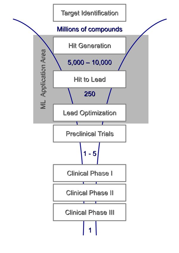
Abstract
The experimental assessment of absorption, distribution, metabolism, excretion, toxicity and
related physiochemical properties of small molecules is counted among the most time- and
cost-intensive tasks in chemical research. Computational approaches, such as machine learn-
ing methods, represent an economic alternative to predict these properties, however, the
limited accuracy and irregular error rate of these predictions restrict their use within the re-
search process. This thesis introduces and evaluates new ideas to enhance the acceptance
and usage of kernel-based machine learning models in chemical research.
The first part of the thesis investigates different approaches to improve the quality of ma-
chine learning predictions in drug discovery. By taking the precise chemical application into
account we derive a new virtual screening algorithm, StructRank, which enables to focus on
the correct ranking of compounds with high binding affinities. Then, the limits of single and
ensemble learning methods are analyzed in the context of hERG inhibition. Since the drug
discovery process often requires the assessment of new chemical series different to previ-
ously examined structures, we introduce and evaluate a clustered cross-validation scheme
that stresses the extrapolation capacity of models. We present a local bias correction to in-
corporate new measurements efficiently and without the need for model retraining.
The second part of the thesis is concerned with two different approaches to assess the re-
liability and interpretability of kernel-based prediction models. The first approach builds
on the visual interpretation of predictions based on the most relevant training compounds.
A compact method to calculate the impact of training compounds on single predictions is
derived and the resulting visualizations are evaluated in a questionnaire study. The second
approach addresses interpretability in terms of chemical features. Here, local gradients are
employed to measure the local influence of specific chemical features on a predicted prop-
erty. The capacity of this approach to identify local as well as global trends in Ames muta-
genicity data, and, to reveal unique characteristics of compound classes such as steroids is
depicted. Finally, we show that the potential of the developed methods extends beyond drug
discovery by using local gradients to enhance the assessment of reaction rates in transition
state theory.
While computational chemistry remains a challenging field of application for machine learn-
ing, the present work introduces methods to improve and assess the quality of machine
learning predictions in order to increase the usage of these methods in chemical research.
Zusammenfassung
Die Untersuchung komplexer pharmakokinetischen Eigenschaften, wie Absorption, Dispo-
sition, Metabolismus oder Toxizität, ist bei Arzneistoffen mit einem enormen experimentel-
len Aufwand und erheblichen Kosten verbunden. Computergestützte Vorhersageverfahren,
wie maschinelle Lernverfahren, können diese Eigenschaften vorhersagen und stellen somit
eine effiziente Alternative zum experimentellen Ansatz dar. Allerdings werden diese Ver-
fahren aufgrund ihrer oft unklaren und wechselhaften Genauigkeit nur zögerlich einge-
setzt. Ziel dieser Arbeit ist es, die Akzeptanz und die Anwendungsmöglichkeiten von
maschinellen Lernverfahren in der chemischen Forschung zu erweitern.
Im ersten Teil der Arbeit steht die Verbesserung von kernbasierten maschinellen Lenver-
fahren in Bezug auf die Anwendungen in der Wirkstoffforschung im Vordergrund. Im er-
sten Kapitel wird ein neuer Algorithmus, StructRank, für das virtuelle Screening entwickelt.
Dieser Algorithmus ist ideal an die Anforderungen des virtuellen Screenings angepasst, da
er eine Rangordnung von Molekülen vorhersagt und Moleküle mit einer hohen Bindungs-
affinität besonders stark berücksichtigt. Das zweite Kapitel beschäftigt sich mit dem Ver-
gleich und der Kombination von Lernverfahren zu einem leistungsstärkeren Ensemble. An-
hand von Daten zur Inhibition des hERG Rezeptors werden die Grenzen und Möglichkeiten
verschiedener Verfahren untersucht. Eine lokale Bias-Korrektur kristallisiert sich hierbei als
ein schnelles und effizientes Verfahren zur Einbindung neuer Messergebnisse ohne erneute
Anpassung des Modells heraus. Im Rahmen dieser Studie wird auch ein neues Kreuz-
Validierungs-Schema untersucht, welches das Extrapolationsvermögen von Prädiktionsmo-
dellen stärker berücksichtigt. Das Extrapolationsvermögen ist in der chemischen Forschung
von besonderer Bedeutung, da die neu zu untersuchenden Verbindungen sich oftmals deut-
lich von allen zuvor untersuchten Molekülen unterscheiden.
Im zweiten Teil der Arbeit werden neue Ansätze zur Bewertung und Interpretation com-
putergestützter Vorhersagen untersucht. Zunächst wird ein Verfahren zur Berechnung des
Einflusses einzelner Trainingsdatenpunkte auf eine Vorhersage hergeleitet. Anschließend
werden die einflussreichsten Verbindungen als Erklärungshilfen zusammen mit der Vorher-
sage visualisiert und dieser Erklärungsansatz in einer empirischen Studie evaluiert. Lokale
Gradienten repräsentieren einen zweiten neuen Ansatz zur Interpretation von Vorhersagen.
Sie messen den lokalen Einfluss einzelner chemischer Eigenschaften auf die Vorhersage.
Mit diesem Verfahren werden sowohl globale als auch lokale Tendenzen auf einem Daten-
satz zur Ames Mutagenität erfasst und Besonderheiten von Verbindungsklassen, wie z.B.
Steroiden identifiziert. Eine Studie zur Berechnung von Reaktionsraten mit Hilfe von lokalen
Gradienten im Rahmen der Theorie des Übergangszustandes verdeutlicht abschießend die
Relevanz der erarbeiteten Verfahren außerhalb der Wirkstoffforschung.
Insgesamt beinhaltet diese Arbeit neue Ideen und Methoden zur Beurteilung und Verbesse-
rung von maschinellen Lernverfahren, um die Anwendungsmöglichkeiten dieser Verfahren
in der chemischen Forschung nachhaltig zu erweitern.
Acknowledgements
First of all, I would like to thank Prof. Dr. Klaus-Robert Müller for giving me the opportu-
nity to work in his group. His infectious optimism and encouragement was of indispensable
value in the course of my research. Prof. Dr. Gisbert Schneider supported me with his exper-
tise in the area of chemoinformatics and I am very grateful to him and his group, including
Dr. Petra Schneider, Tim Geppert and Felix Reisen, for introducing me to the experimental
side of chemoinformatics.
This work would not have been possible without the contributions of my coworkers and
colleagues. Dr. Timon Schroeter, who talked me into chemoinformatics, gave me inspiration
and motivation for my research. I would like to thank Dr. Matthias Rupp for his thorough
review of my work and his reliable assistance within the past year. A great thanks goes to
David Baehrens, Fabian Rathke, Dr. Ulf Brefeld and Peter Vascovic for their help on design-
ing and implementing new algorithms. I would like to thank my collaborators at Idalab,
Bayer Schering Pharma and Boehringer Ingelheim, especially Dr. Sebastian Mika, Dr. Anto-
nius ter Laak, Dr. Nikolaus Heinrich, Dr. Andreas Sutter and Dr. Jan Kriegl, for many fruitful
discussions and the open exchange of experience. The participants of ”Navigation Chemical
Compound Space for Materials and Bio Design” program at IPAM, UCLA inspired my work
and I would like to thank Zachary Pozun, John Snyder, Prof. Dr. Kieron Burke, Dr. Daniel
Sheppard and Prof. Dr. Graeme Henkelman for their calculations and willingness to share
their knowledge.
I deeply enjoyed working at the Machine Learning Group of the Berlin Institute of Technol-
ogy and would like to thank all members for generating a kind and open-minded research
atmosphere. A special thanks goes to my former office mates Dr. Tobias Lang, Stanimı́r
Dragı́ev and Martijn Schreuder. Their humor and friendship was always a great support.
I gratefully acknowledge the funding from the German Research Foundation (MU 987/4-2),
the German Academic Exchange Service and the European Commission under the PASCAL2
Network of Excellence of the FP7-ICT program.
Finally, I would like to thank my family and friends who, non-scientifically but to the same
degree, supported my work. In particular I would like to express my gratitude to the group
of women which originated from the ProMotion program, to Annika who fostered my inter-
est in life science and, most of all, to Marcel for his patience and understanding.
Contents

Preface                                                                                                                              iii

1   Introduction                                                                                                                      1
    1.1 Machine Learning . . . . . . . . . . . . . . . . . . . .         .   .   .   .   .   .   .   .   .   .   .   .   .   .   .    1
    1.2 Chemoinformatics and the Drug Discovery Process                  .   .   .   .   .   .   .   .   .   .   .   .   .   .   .    2
    1.3 Machine Learning in Drug Discovery . . . . . . . .               .   .   .   .   .   .   .   .   .   .   .   .   .   .   .    4
         1.3.1 Thesis Scope and Contributions . . . . . . .              .   .   .   .   .   .   .   .   .   .   .   .   .   .   .    5

2   Ranking Approach to Virtual Screening                                                                                             7
    2.1 Introduction . . . . . . . . . . . . . . . . . . . . . . . .         .   .   .   .   .   .   .   .   .   .   .   .   .   .    7
    2.2 Methods . . . . . . . . . . . . . . . . . . . . . . . . . .          .   .   .   .   .   .   .   .   .   .   .   .   .   .    8
        2.2.1 Evaluate Rankings Using NDCG . . . . . . . .                   .   .   .   .   .   .   .   .   .   .   .   .   .   .    8
        2.2.2 Structured Support Vector Machines for QSAR                    .   .   .   .   .   .   .   .   .   .   .   .   .   .    9
        2.2.3 Baseline Models . . . . . . . . . . . . . . . . . .            .   .   .   .   .   .   .   .   .   .   .   .   .   .   10
        2.2.4 Further Approaches and Alternatives . . . . .                  .   .   .   .   .   .   .   .   .   .   .   .   .   .   12
    2.3 Data . . . . . . . . . . . . . . . . . . . . . . . . . . . . .       .   .   .   .   .   .   .   .   .   .   .   .   .   .   13
        2.3.1 Descriptor Generation and Data Preparation .                   .   .   .   .   .   .   .   .   .   .   .   .   .   .   13
        2.3.2 Test Framework . . . . . . . . . . . . . . . . . .             .   .   .   .   .   .   .   .   .   .   .   .   .   .   14
        2.3.3 Alternative Performance Measures . . . . . . .                 .   .   .   .   .   .   .   .   .   .   .   .   .   .   15
        2.3.4 Toy Example . . . . . . . . . . . . . . . . . . .              .   .   .   .   .   .   .   .   .   .   .   .   .   .   15
    2.4 Results . . . . . . . . . . . . . . . . . . . . . . . . . . .        .   .   .   .   .   .   .   .   .   .   .   .   .   .   16
        2.4.1 Virtual Screening Datasets . . . . . . . . . . . .             .   .   .   .   .   .   .   .   .   .   .   .   .   .   16
        2.4.2 Toy Example . . . . . . . . . . . . . . . . . . .              .   .   .   .   .   .   .   .   .   .   .   .   .   .   17
        2.4.3 Run Time Comparison . . . . . . . . . . . . . .                .   .   .   .   .   .   .   .   .   .   .   .   .   .   18
    2.5 Discussion . . . . . . . . . . . . . . . . . . . . . . . . .         .   .   .   .   .   .   .   .   .   .   .   .   .   .   19

3   Optimal Combination of Models                                                                                                    21
    3.1 Introduction . . . . . . . . . . . . . . . . . . . . . .     .   .   .   .   .   .   .   .   .   .   .   .   .   .   .   .   21
    3.2 Data . . . . . . . . . . . . . . . . . . . . . . . . . . .   .   .   .   .   .   .   .   .   .   .   .   .   .   .   .   .   22
        3.2.1 Molecular Descriptors & Pre-Processing . .             .   .   .   .   .   .   .   .   .   .   .   .   .   .   .   .   22
        3.2.2 Comparison of in-house and literature data             .   .   .   .   .   .   .   .   .   .   .   .   .   .   .   .   23
        3.2.3 Analysis of Outliers . . . . . . . . . . . . .         .   .   .   .   .   .   .   .   .   .   .   .   .   .   .   .   23
    3.3 Methods . . . . . . . . . . . . . . . . . . . . . . . .      .   .   .   .   .   .   .   .   .   .   .   .   .   .   .   .   24
        3.3.1 Single Modeling Approaches . . . . . . . .             .   .   .   .   .   .   .   .   .   .   .   .   .   .   .   .   24
        3.3.2 Ensemble Modeling Approaches . . . . . .               .   .   .   .   .   .   .   .   .   .   .   .   .   .   .   .   25
    3.4 Evaluation Strategy . . . . . . . . . . . . . . . . . .      .   .   .   .   .   .   .   .   .   .   .   .   .   .   .   .   27
        3.4.1 Evaluation of Single Models . . . . . . . . .          .   .   .   .   .   .   .   .   .   .   .   .   .   .   .   .   27
        3.4.2 Evaluation of Ensemble Models . . . . . .              .   .   .   .   .   .   .   .   .   .   .   .   .   .   .   .   27
    3.5 Results and Discussion . . . . . . . . . . . . . . . .       .   .   .   .   .   .   .   .   .   .   .   .   .   .   .   .   28
        3.5.1 Single Models . . . . . . . . . . . . . . . . .        .   .   .   .   .   .   .   .   .   .   .   .   .   .   .   .   28
        3.5.2 Ensemble Models . . . . . . . . . . . . . . .          .   .   .   .   .   .   .   .   .   .   .   .   .   .   .   .   31
    3.6 Conclusions . . . . . . . . . . . . . . . . . . . . . .      .   .   .   .   .   .   .   .   .   .   .   .   .   .   .   .   33

                                                  i
Contents
4 Structure-based Explanation of Nonlinear Classifiers 37
4.1 Interpretability of Predictions in Chemoinformatics . . . . . . . . . . . . . . . 37
4.2 The Idea of Structure-Based Explanations . . . . . . . . . . . . . . . . . . . . . 38
4.3 Measuring Influence in Predictions of Kernel-Based Models . . . . . . . . . . 39
4.4 Evaluation of Compound Relevance Weights . . . . . . . . . . . . . . . . . . . 40
4.5 Related Work . . . . . . . . . . . . . . . . . . . . . . . . . . . . . . . . . . . . . 43
4.6 Discussion . . . . . . . . . . . . . . . . . . . . . . . . . . . . . . . . . . . . . . . 44
4.7 Conclusions . . . . . . . . . . . . . . . . . . . . . . . . . . . . . . . . . . . . . . 47
5 Interpretation in Terms of Local Feature Importance 49
5.1 Methods . . . . . . . . . . . . . . . . . . . . . . . . . . . . . . . . . . . . . . . . 49
5.2 Evaluation of Explanation Vectors . . . . . . . . . . . . . . . . . . . . . . . . . 53
5.3 Related Work . . . . . . . . . . . . . . . . . . . . . . . . . . . . . . . . . . . . . 56
5.4 Discussion . . . . . . . . . . . . . . . . . . . . . . . . . . . . . . . . . . . . . . . 57
5.5 Conclusions . . . . . . . . . . . . . . . . . . . . . . . . . . . . . . . . . . . . . . 58
6 Learning Transition States 59
6.1 Introduction . . . . . . . . . . . . . . . . . . . . . . . . . . . . . . . . . . . . . . 59
6.2 Transition State Surface Estimation via Binary Classification . . . . . . . . . . 61
6.3 Experiments and Results . . . . . . . . . . . . . . . . . . . . . . . . . . . . . . . 62
6.4 Discussion and Conclusions . . . . . . . . . . . . . . . . . . . . . . . . . . . . . 65
A Overview of Machine Learning Methods & Concepts 69
A.1 Empirical Risk Minimization . . . . . . . . . . . . . . . . . . . . . . . . . . . . 69
A.2 Standard Machine Learning Approaches . . . . . . . . . . . . . . . . . . . . . . 72
A.3 Model Evaluation . . . . . . . . . . . . . . . . . . . . . . . . . . . . . . . . . . . 75
B Abbreviations 77
iiPreface
Machine learning (ML) is a branch of artificial intelligence concerned with the development
of cost-efficient computing systems with learning capability. Nowadays these systems can
be found in automated mail sorting programs, voice-controlled writing applications, recom-
mender system of online stores like Amazon, computer firewalls and many other parts of
our everyday live. Especially data-rich areas of science like bioinformatics, image process-
ing or neuroscience benefit from the automated knowledge acquisition of machine learning
algorithms.
In chemistry, machine learning algorithms are predominantly employed in the area of drug
discovery. Nonlinear machine learning methods like support vector machines, neural net-
works, random forests, and Gaussian processes can be used to predict ADMET (absorption,
distribution, metabolism, excretion, and toxicity) and related physicochemical properties
[89, 48, 29, 115, 113]. In drug discovery an early assessment of these properties is highly im-
portant in order to prioritize compounds thereby save costs, time and controversial animal
experiments.
Due to the complexity of chemical systems, the vast space of chemical compounds and the
limited amount of experimental data, however, current approaches fail to provide predic-
tion models of general accuracy for complex chemical properties. Moreover, there exist no
accurate confidence estimates for the single predictions of these systems. Thus, machine
learning methods find only limited application in industrial research and can support, but
not substitute laboratory experiments.
This thesis aims to extend the acceptance and usability of kernel-based machine learning
methods in chemical research. Based on a close analysis of chemical problems and experi-
mental data, we derive new algorithms and methods to enhance machine learning predic-
tions and to asses their reliability.
iiiChapter 0. Preface
Roadmap
CHAPTER 1 The first chapter gives a brief introduction to chemoinformatics, drug discov-
ery and machine learning. The special requirements of machine learning methods arising in
chemical applications are discussed and related to the author’s contributions.
CHAPTER 2 In the second chapter we build on the framework of structured-learning and a
metric used in information retrieval to derive a novel algorithm for virtual screening. In con-
trast to previous approaches this algorithm directly ranks compounds and focuses strongly
on high binding affinities. The capability of the new algorithm StructRank is illustrated on
three different screening datasets with different label distributions.
CHAPTER 3 This chapter is concerned with ensemble models and local correction ap-
proaches in the context of hERG inhibition. Moreover, a typical research scenario, where the
compounds of interest are not directly related to the training data, is simulated in order to ex-
amine the differences between standard and the newly introduced clustered cross-validation
framework.
The second part of this thesis investigates methods to assess the reliability and applicability
of ML predictions:
CHAPTER 4 A visual approach to explaining kernel-based predictions is introduced. The
most relevant training compounds are visualized along with the predicted value in order to
allow for an intuitive understanding and interpretation of single predictions. A question-
naire study on Ames mutagenicity prediction is performed to illustrate how this approach
can help to spot wrong labels, detect poor model applicability and discover important chem-
ical characteristics of the training data.
CHAPTER 5 In the fifth chapter local gradients are used to measure the local importance
of chemical features in nonlinear classification models. The relevance of local gradients for
chemical prediction models is illustrated on Ames mutagenicity data. The results reveal that,
in contrast to common feature importance measures, this new approach allows to detect local
as well as global trends within chemical data.
CHAPTER 6 Support vector machines and local gradients are introduced to transition state
theory. We demonstrate how these methods can improve the assessment of the transition
surface and reaction rates.
ivPreviously Published Work
Parts of this thesis have been discussed in previous journal publications (co)authored by the
author of this thesis:
• Anton Schwaighofer, Timon Schroeter, Sebastian Mika, Katja Hansen, Antonius ter
Laak, Philip Lienau, Andreas Reichel, Nikolaus Heinrich and Klaus-Robert Müller A
Probabilistic Approach to Classifying Metabolic Stability. Journal of Chemical Information
and Modelling, 48(4): 785-796, 2008.
• Katja Hansen, Sebastian Mika, Timon Schroeter, Andreas Sutter, Antonius ter Laak,
Thomas Steger-Hartmann, Nikolaus Heinrich and Klaus-Robert Müller. Benchmark
Data Set for in Silico Prediction of Ames mutagenicity. Journal of Chemical Information
and Modelling, 49(9): 2077-2081, 2009. (Chapter 4 and 5)
• Katja Hansen, Fabian Rathke, Timon Schroeter, Georg Rast, Thomas Fox, Jan M. Kriegl
and Sebastian Mika. Bias-Correction of Regression Models: A Case Study on hERG Inhibi-
tion. Journal of Chemical Information and Modelling, 49(6):1486-1496, 2009. (Chapter
1 and 3)
• Matthias Rupp, Timon Schroeter, Ramona Steri, Heiko Zettl, Ewgenij Proschak, Katja
Hansen, Oliver Rau, Oliver Schwarz, Lutz Müller-Kuhrt, Manfred Schubert-Zsilavecz,
Klaus-Robert Müller and Gisbert Schneider. From machine learning to natural product
derivatives selectively activating transcription factor PPARγ . ChemMedChem,Wiley, 5(2):
191-194, 2010.
• Ramona Steri, Matthias Rupp, Ewgenij Proschak, Timon Schroeter, Heiko Zettl, Katja
Hansen, Oliver Schwarz, Lutz Müller-Kuhrt, Klaus-Robert Müller, Gisbert Schneider
and Manfred Schubert-Zsilavecz. Truxillic acid derivatives act as peroxisome proliferator-
activated receptor y activators. Bioorganic & Medicinal Chemistry Letters, 20: 29202923
2010.
• David Baehrens, Timon Schroeter, Stefan Harmeling, Motoaki Kawanabe, Katja Hansen
and Klaus-Robert Müller. How to Explain Individual Classification Decisions. Journal of
Machine Learning Research, 11: 1803-1831, 2010. (Chapter 5)
• Iurii Sushko, Sergii Novotarskyi, Robert Korner, Anil Kumar Pandey, Artem Cherkasov,
Jiazhong Li, Paola Gramatica, Katja Hansen, Timon Schroeter, Klaus-Robert Müller,
Lili Xi, Huanxiang Liu, Xiaojun Yao, Tomas Oberg, Farhad Hormozdiari, Phuong Dao,
Cenk Sahinalp, Roberto Todeschini, Pavel Polishchuk, Anatoliy Artemenko, Victor
Kuzmin, Todd M. Martin, Douglas M. Young, Denis Fourches, Eugene Muratov, Alexan-
der Tropsha, Igor Baskin, Dragos Horvath, Gilles Marcou, Christophe Muller, Alexan-
der Varnek, Volodymyr V. Applicability domains for classification problems: Benchmarking
of distance to models for Ames mutagenicity set. Journal of Chemical Information and
Modelling, 50(12): 2094-111, 2010.
• Katja Hansen, David Baehrens, Timon Schroeter, Matthias Rupp and Klaus-Robert
Müller. Visual Interpretation of Kernel-Based Prediction Models. Molecular Informatics,
30: 817-826 2011. (Chapter 4)
• Fabian Rathke, Katja Hansen, Ulf Brefeld and Klaus-Robert Müller. StructRank: A New
Approach for Ligand-Based virtual screening. Journal of Chemical Information and Mod-
elling, 51(1): 83-92 2011. (Chapter 2)
• Zachary D. Pozun, Katja Hansen, Daniel Sheppard, Matthias Rupp, Klaus-Robert Müller
and Graeme Henkelman. Optimizing Transition State Dividing Surfaces via Kernel-Based
Machine Learning, submitted. (Chapter 6)
vChapter 0. Preface
• Grigorios Skolidis, Katja Hansen, Guido Sanguinetti and Matthias Rupp. Multi-task
learning for pK a prediction, submitted.
• John C. Snyder, Matthias Rupp, Katja Hansen, Klaus-Robert Müller and Kieron Burke.
Finding Density Functionals with Machine Learning, submitted.
viChapter 1
Introduction
1.1 Machine Learning
The field of machine learning (ML) seeks to infer and generalize dependencies from data
using computing systems with learning capability. ML is concerned with many research
questions arising in the field of statistics, data mining and psychology, but with differences
of emphasis. Statistics focuses on understanding the data generating process, often with
the goal of testing hypotheses, whereas data mining seeks to find patterns in the data and
psychological studies aspire to understand the mechanisms underlying human learning be-
haviors [26]. In contrast, the machine learning methods investigated in the following are
primarily concerned with predictive modeling, where a model is built to mimic and gen-
eralize a certain characteristic of the data generating process. More precisely, the goal is to
predict the label y for some test sample x by taking a given training set D into account.
Types of Learning
The training set D may consist of
• samples with associated labels (supervised learning scenario),
• solely of samples without labels (unsupervised learning scenario),
• labeled and unlabeled samples (semi-supervised learning scenario).
Within this thesis, we focus on supervised learning scenarios. The training sets usually con-
sist of small molecules represented as vectors of chemical descriptors with associated exper-
imental measurements of physical or chemical properties. The constitution of the measure-
ment values y determines the type of learning task: Quantitative measurements result in
regression tasks, whereas classification tasks are determined by qualitative measurements. The
class of ranking tasks discussed in Chapter 2 forms an exception where the labels are contin-
uous values as in regression tasks but the prediction is a ranking of compounds according
to their unknown labels.
The Frequentist and the Bayesian Approach
A fundamental basis of machine learning is statistical inference, i.e. the process of drawing
conclusions from observable data that are subject to random variation. There are two differ-
ent views on inference in statistics resulting from different definitions of probability.
1Chapter 1. Introduction
For a frequentist a statistical model equals a function y = f (x; θ), where f represents a class
of parametric functions with parameters θ processing input sample x. The strategy for learn-
ing is based on determining the parameters θ such that f is optimal with respect to certain
likelihood terms or loss functions.
From a Bayesian point of view the parameters θi are not fixed but distributed according to a
known prior distribution P (θ). An initial model is designed based on this prior information
and then adapted in light of the observed data. The model provides a representation of our
prior knowledge about the system and the information derived from the data [8]. Thus the
prediction takes the form of a predictive distribution P (y|x) which can be interpreted as an
expression of our degrees of belief in the various possible outcomes y [83].
Over the last decades a huge amount of research publications addressed machine learning
and respective theory, building on the work of Vapnik [138] and Rosenblatt [100]. The Ap-
pendix provides an overview of the main concepts and ideas of the machine learning meth-
ods implemented in this thesis. For a comprehensive introduction into the field of machine
learning we refer to the literature [46, 8, 81, 28] for further reading.
1.2 Chemoinformatics and the Drug Discovery Process
Chemoinformatics
Chemoinformatics (also cheminformatics) is a young research area at the interface of chem-
istry and informatics [148, 36, 13] that employs mathematical and statistical methods to ex-
tract information from chemical data [35]. In the 1970’s chemists started to discover comput-
ers as tools for chemical research. From the very beginning, however, it could be observed
that there was a split between theoretical chemists using computers for quantum mechani-
cal calculations and chemists using computers for information processing and data analysis
[36]. The first group of theoretical chemists founded the research area of computational
chemistry, while the latter group denominated their research as chemoinformatics. The two
fields, however, are highly related and the differences only vaguely defined.
In chemoinformatics machine learning methods are predominantly applied to problems aris-
ing in the context of drug discovery and design. However, as exemplified in Chapter 6, the
field of theoretical chemistry provides opportunities for machine learning as well.
Drug Discovery Process
The drug discovery and development process of a single new drug encompasses between
ten and fifteen years of research and costs about 1.8 billion dollars (Paul et al. [91]).
The first step in drug discovery comprises the selection and confirmation of a target, a single
molecule, often a protein, which is involved in the disease mechanism and can potentially
interact with a drug molecule to affect the disease. In the following screening step one seeks
to find hits, small molecules that interact with the target. The most common approach is
high-throughput screening (HTS) where screening robots are used to perform a chemical
assay on millions of compounds. Alternatively, virtual screening or molecular modeling
techniques are applied. Here, computational methods (in silico methods) are implemented to
assess the potential of compounds.
After the effect of the identified hits on the target has been confirmed in laboratory exper-
iments, the first safety tests are performed on the most promising compounds (hit-to-lead
phase). ADMET (absorption, distribution, metabolism, excretion, and toxicity) and related
21.2. Chemoinformatics and the Drug Discovery Process
Figure 1.1: Sketch of the drug discovery process.
properties are investigated in order to exclude dangerous side effects. The most promising
compounds are then determined as leads.
During lead optimization these lead structures are modified to improve efficacy and en-
hance their ADMET profile. A successful drug needs to be absorbed into the bloodstream,
distributed to the proper organs, metabolized efficiently and effectively and then be excreted
from the body without any toxic side effects. The mutual optimization of these highly related
drug properties is the key challenge in lead optimization. Finally, about 2% of the originally
identified hits enter the preclinical trials where laboratory and animal experiments are per-
formed to determine if the compound is safe enough for human testing.
The subsequent phases of clinical trials are denoted as the drug development process. Starting
from groups of 20 to 100 healthy volunteers (phase 1) over small groups of patients (phase
2) to large studies including 1,000 to 5,000 of patients (phase 3) the drug candidate is exten-
sively tested to determine risks, efficacy and dosing. A successful drug candidate is then
approved as new drug and enters the market.
A key problem of todays pharmaceutical industry is the productivity of this drug develop-
ment process [91]. While the number of newly approved innovative drugs is decreasing the
loss of revenues due to patent expirations for successful products and rising development
costs are limiting research activities [39]. Following the “fail early—fail cheap” paradigm,
companies now try to consider ADMET properties (using e.g. ML methods) as early as pos-
sible in the drug development process.
3Chapter 1. Introduction
1.3 Machine Learning in Drug Discovery
Different areas within drug discovery benefited from utilizing machine learning technolo-
gies (see Wale [142] for a review). Among them are:
• Virtual screening: In virtual screening machine learning techniques are applied to rank
or filter compounds with respect to different properties (Melville et al. [79] reviews ap-
plications in ligand-based and structure-based virtual screening). Especially in ligand-
based virtual screening, where no structural information about the target is available,
machine learning methods enhance similarity search—even if only very few reference
compounds are given [50]. Additionally, ML methods may be applied to create diverse
compound libraries that can serve as input for virtual screening (library design) [105].
• Quantitative structure-activity relationship (QSAR) and quantitative structure-property
relationship (QSPR): QSAR and QSPR models are statistical models used to infer de-
pendencies between chemical structures and their biological activity or physicochem-
ical properties. Within the last decades machine learning models like neural networks
or support vector machines became popular in this area of research.
• Prediction of protein structure, function and interaction: Machine learning methods
have found extensive applications in biochemical tasks like protein structure predic-
tion, protein function prediction and characterization of protein-protein interaction.
Though these problems are related to drug discovery, we will subsequently restrict
ourselves solely to machine learning applications on drug-like compounds. However,
most of the challenges discussed in the following occur in all three areas of application.
Challenges of ML in Drug Discovery
In order to generate an operational prediction model for chemical applications multiple chal-
lenges of chemical data have to be addressed, mainly:
Representation of chemical structures
Chemical compounds are flexible three-dimensional structures that change shape and
conformation as they interact with the environment. In order to apply statistical meth-
ods, the compounds are represented as vectors of molecular descriptors. These num-
bers reflect shape, charge, connectivity, weight and various other properties derived
from the 2D and/or 3D structure of the molecules [131]. Some methods also allow
to work directly on the 2D or 3D graph structures by using, e.g., graph kernels [101].
Unfortunately, both approaches are not able to capture the flexibility of molecules and
the special characteristics of chemical compounds exhibiting several graph structures
(tautomers) or several 3D structures (conformers) are not considered.
Constitution of empirical measurements:
A collection of empirical data like laboratory measurements is exposed to different
sources of error: inaccurate labeling, systematic measurement errors and the inherent
error of the measuring system. Thus, each modeling approach requires a thorough
pre-processing including outlier analysis, visual data inspection and if necessary nor-
malization.
Amount and distribution of data:
In early stages of the drug discovery process there is little knowledge about the target
and the available datasets are small and of low diversity. Prediction models build on
this kind of data are prone to overfitting and show a low generalization capacity.
41.3. Machine Learning in Drug Discovery
Though the dataset grows stepwise with the ongoing development, the newly inves-
tigated compounds commonly lie beyond previously examined series of compounds.
Thus, prediction results stay inaccurate due to missing information in the chemical
space of interest.
Complexity of chemical interactions:
Machine learning in drug discovery relies on the assumption that similar molecules
exhibit similar activity. This implies that the activity value changes continuously over
chemical space and can be pictured as a smooth surface. Unfortunately, very similar
compounds may in some cases possess extremely different activities leading to rugged
canyons called “activity cliffs” in the activity landscape [76]. The detection and mod-
eling of such activity cliffs is a problem of ongoing research.
On the one hand it is highly desirable to strive for a statistical model meeting all these chal-
lenges (and a lot of ongoing research addresses these problems). On the other hand one
has to keep in mind that it is unrealistic to find such a model. Chemists and physicists are
still discovering new chemical phenomena and modes of molecular interaction. Our current
chemical knowledge is somehow incomplete and we can not expect a perfect model on the
basis of incomplete information.
Thus, the question arises how to deal with the imperfection of data in chemoinformatics
and the resulting inaccuracy of prediction models. In the following chapters this problem is
addressed from an use-oriented point of view.
1.3.1 Thesis Scope and Contributions
In the first part of this thesis we analyze how one can incorporate the limited amount of data
in a (kernel-based) prediction model such that it optimally fits the conditions and require-
ments of virtual screening and lead optimization.
Virtual screening aims to rank molecules in terms of their binding coefficients for the inves-
tigated drug target, such that the top-k molecules can be selected for further investigation.
Thus, we derive a new screening algorithm StructRank which directly predicts a ranking for a
given set of compounds and allows to focus on high binding affinities (Chapter 2). In con-
trast to other ligand-based screening algorithms the new approach is based on the relative
binding affinity and makes better use of the information encoded in the training data if only
few highly binding compounds are available.
In lead optimization and hit-to-lead optimization the exact prediction of chemical proper-
ties related to unfavorable side-effects is required. With every new batch of experiments
more training data becomes available but the requested predictions commonly concern new
molecules beyond this dataset. To estimate the prediction accuracy in such an application
scenario we present a clustered cross-validation scheme (Section 3.4.1 and A.3) and compare it
to standard cross-validation. Moreover, we show how the newly received data can be ben-
eficially incorporate using local bias correction (Chapter 3). On the basis of hERG inhibition
data this method is evaluated and compared to ensemble learning approaches.
The introduced methods significantly improve prediction models by extracting the most
relevant information of a given (incomplete) dataset with respect to a certain application in
drug discovery. Nevertheless, they can not reach perfect accuracy and a validity measure for
single predictions is needed in order to to prioritize compounds correctly within the research
process.
Thus the second part of this thesis is dedicated to the interpretability, knowledge of the do-
5Chapter 1. Introduction
main of applicability1 , and estimation of confidence in machine learning based predictions.
In Chapter 4 we develop and validate a method for the interpretation of kernel-based prediction
models. The most influential training compounds are identified and visualized for individ-
ual predictions as foundation of interpretation. As a consequence of this interpretability,
the method helps to assess regions of insufficient coverage or activity cliffs, to spot wrong
labeling, and to determine relevant molecular features as illustrated on Ames mutagenicity
data.
Subsequently, local gradients are introduced as a tool for interpretation in terms of chemical
features (Chapter 5). They facilitate the understanding of prediction models by indicating
the chemical input features with the greatest impact on the predicted value. Given a well-
founded prediction model the local gradients allow to deduce global and local structure
elements of the chemical space and thereby facilitate compound optimization. The frame-
work presented and evaluated in Chapter 5 allows to calculate such local gradients for any
classification model.
Finally, we illustrate the utility of the developed methods beyond drug discovery and de-
sign. Transition state theory is known as a semi-classical approach to assess the transition
surface and reaction rate within the field of theoretical chemistry. In Chapter 6 support vec-
tor machines and local gradients are for the first time applied to enhance the sampling of
the potential energy surface. The new sampling approach accelerates the assessment of the
transition surface and improves the resulting reaction rate.
1
The domain of applicability of a model refers to the part of the chemical space where the model provides
reliable predictions.
6Chapter 2
A Ranking Approach for
Ligand-Based Virtual Screening
2.1 Introduction
Screening large libraries of chemical compounds against a biological target, typically a re-
ceptor or an enzyme, is a crucial step in the process of drug discovery.
Besides high-throughput screening, the physical screening of large libraries of chemicals,
computational methods, known as virtual screening (VS), [144] gained attention within the
last two decades and were applied successfully as an alternative and complementary screen-
ing tool [93, 102].
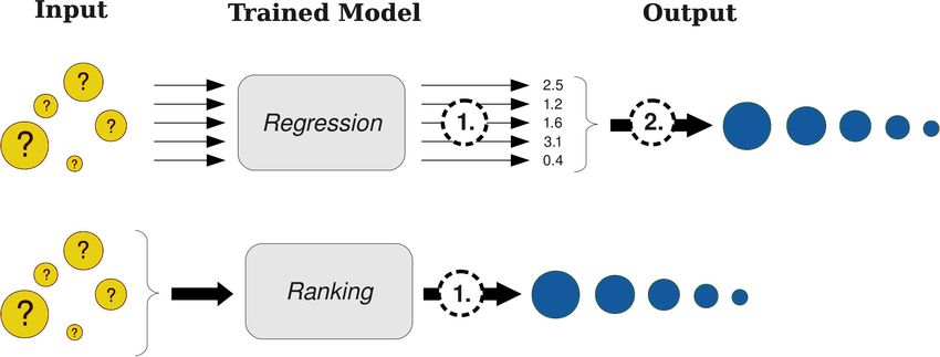
The task in VS, also known as “early recognition problem” [136, 84], can be characterized
as follows: Given a library of molecules, the task is to output a ranking of these molecules
in terms of their binding coefficient for the investigated drug target, such that the top k
molecules can be selected for further investigations. As a standard, current quantitative
structure-activity relationship (QSAR) regression models are applied to predict the level of
activity: They learn a function f : x 7→ y, f : Rd → R that predicts a label for any molecule
given its features. To establish the subset of candidate molecules, predictions are made for
all molecules in the database. In a second step an ordered list is generated based on these
predictions. This two step approach is shown in Figure 2.1 (top). Finally the top k ranked
compounds are selected to be investigated in more detail.
Figure 2.1: Two different ways to solve the ranking task of virtual screening: a) State-of-the-
art approaches use a 2-step approach. In the first step a regression model is used to predict
binding coefficients for all molecules in the library. In a second step the molecules are sorted
according to their predictions. b) The new ranking approach directly predicts the ranking
within a single step.
7Chapter 2. Ranking Approach to Virtual Screening
However, virtual screening approaches primarily aim to find molecules exhibiting high
binding affinities with the target while the predictive accuracy with respect to the labels
y is only of secondary interest. Although a perfect regression model would also imply a per-
fect ranking of the molecules of interest, the impact of suboptimal regressors on the ranking
is not easily captured as equal models in terms of their mean squared error could give rise
to completely different rankings. Thus, the question rises whether the detour via regression
is necessary and whether the task can be addressed in a more natural way. In this chapter, a
top k ranking algorithm, StructRank, that directly solves the ranking problem and that focuses
on the most promising molecules (cf. 2.1, bottom) is derived and evaluated on three virtual
screening datasets.
2.2 Methods
The formal problem setting of ranking for virtual screening is as follows: Let {(xi , yi )ni=1 } be
a given set of n molecules, where xi ∈ Rd denotes the feature vector of the i-th molecule con-
taining the molecular descriptors, and yi ∈ R is a scalar representing the biological/chemical
property of that molecule, e.g. binding affinity.
Based on this set we aim at learning a function f : X → P that takes any set of molecules
x̃ = {x1 , . . . , xm } ∈ X and returns a ranking p ∈ P 1 of these molecules according to the bio-
logical/chemical property of interest. Moreover, as the purpose of virtual screening methods
is to rank actives early in an ordered list (see “early recognition problem” [136, 84]), we want
the learning machine to focus on the top k molecules in the ranking.
In the following we derive a top k ranking SVM meeting these requirements for QSAR. The
approach builds on work by Chapelle et al. [20] and Tsochantaridis [137].
2.2.1 Evaluate Rankings Using NDCG
The definition of an adequate quality measure for rankings of molecules is of crucial impor-
tance in the development of a ranking algorithm suitable for virtual screening. We propose
to use a popular ranking measure that originates from the information retrieval community:
Normalized Discounted Cumulative Gain (NDCG). Given the true ranking p̄, a predicted
ranking p̂ and a cut-off k, NDCG is given by the DCG (Discounted Cumulative Gain) for the
predicted ranking normalized by the DCG of the true ranking:
k
DCGk (p̂) X 2p[y]r − 1
N DCGk (p̄, p̂) = , DCGk (p) = (2.1)
DCGk (p̄) log2 (1 + r)
r=1
where p[y]r is the binding coefficient yi of the molecule xi ranked at position r.
Originally, NDCG [56] was introduced to evaluate the results of web searches. It measures
how similar a predicted ranking is compared to the true ranking. NDCG has several impor-
tant properties:
• NDCGk only evaluates the first k positions of predicted rankings, thus an error on
positions below rank k is not punished.
• Furthermore the first k positions are weighted, which means that errors have different
influence on the final score depending on which position of the ranking they occur.
1
In the following a ranking is described as a permutation p, i.e. for a given set of molecules x̃ and a vector y
of corresponding binding coefficients, p[y] gives ideally the vector of binding coefficients in decreasing order.
82.2. Methods
Naturally position one is the most important, with lower positions discounted by the
log of their rank r: log2 (1 + r).
• Finally, NDCG is normalized, thus if the predicted ranking equals the true ranking
the score is 1. To translate NDCG into a loss function we simply use ∆(p, p̂) = 1 −
N DCG(p, p̂).
In summary, NDCG aims at pushing the molecules with the highest binding affinity on top
of the ranking.
2.2.2 Structured Support Vector Machines for QSAR
Let us reconsider the ultimate target of learning a function f : X → P that maps a set of
molecules onto a ranking. In order to establish f , we utilize the basic concepts of Structured
SVMs (see Tsochantaridis et al. [137]), a very flexible learning machine that has been applied
to many different learning tasks in information retrieval [20, 152], natural language parsing
[10], and protein sequence alignment [151]. Structured SVMs learn a discriminant function
F : X × P → R. F can be thought of as a compatibility function, that measures how well
a certain ranking p fits the given set of molecules x̃. The final prediction is given by the
ranking p that achieves the maximal score F (x̃, p). Thus we have
f (x̃) = argmax F (x̃, p).
p∈P
F is defined over a combined space of sets of molecules and corresponding rankings, a so
called “joint feature space”. To be able to learn F directly in that combined space, we define
a function Ψ that maps each pair of a set of molecules x̃ together with a ranking p (of x̃) onto
one corresponding data point in the joint feature space
n
X
Ψ(x̃, p) = φ(x̃i )A(pi ) (2.2)
i=1
where the function φ is a mapping into a Hilbert space corresponding to a kernel function
k(xi , xj ) and A(r) = max(0, k + 1 − r) weights the molecules according to their ranks as
proposed by Chapelle [20]. Only molecules corresponding to the first k ranks are incorpo-
rated.
Given the joint feature map Ψ, F is defined as a linear function in the joint feature space:
F (x̃, p) = wT Ψ(x̃, p),
F is the scalar product of the corresponding joint feature map of x̃ given a particular ranking
p and the learned parameter vector w.
Modeling F can be casted as follows: Given a set of molecules x̃ we want the true ranking p̄
to score highest among all possible rankings p ∈ P transforming into constraints
wT (Ψ(x̃, p̄) − Ψ(x̃, p)) ≥ 0 ∀ p ∈ P \ p̄.
Alike classic SVMs for classification [138] this can be turned into a maximum-margin prob-
lem, where we want the difference between the true ranking p̄ and the closest runner-up
argmaxp6=p̄ wT Ψ(x̃, p) to be maximal (cf Section A.2, support vector classification). Also we
want different p’s to get separated according to the degree of their falseness: A predicted
ranking with only two ranks interchanged compared to the true ranking is much better than
a predicted ranking with all ranks interchanged. We thus require the latter to get further sep-
arated with a larger margin from the true ranking than the first one. This is accomplished by
9Chapter 2. Ranking Approach to Virtual Screening
replacing the constant margin formulation with the loss-dependent margin (margin scaling
[137, 127]):
wT (Ψ(x̃, p̄) − Ψ(x̃, p)) ≥ ∆(p, p̄) ∀ p ∈ P \ p̄ (2.3)
where 1-NDCGk is used for ∆(p, p̄). Furthermore a slack variable ξ is introduced that re-
flects the maximal error made for the set of constraints (see eq.(2.3)). Finally, to improve
performance, we employ a boosting approach: We randomly draw m different subsets x̃j of
molecules from the training set. Applying the methodology described so far to each subset
j we obtain the final optimization problem
m
1 T X
min w w+C ξj (2.4)
w,ξ 2
j=1
subject to w (Ψ(x̃ , p̄ ) − Ψ(x̃j , p)) ≥ ∆(p̄j , p) − ξ j
T j j
∀j, ∀p 6= p̄j
ξ j ≥ 0.
The corresponding dual is given by
1
max − αT L α + bT α (2.5)
α
X2
subject to αpj ≤ C, αpj ≥ 0 ∀j, ∀p 6= p̄j
p∈P
where we have an α for each possible ranking p of subset x̃j . The matrix L consists of entries
(L)ip,jp0 = (Ψ(x̃i , p̄i ) − Ψ(x̃i , p))T (Ψ(x̃j , p̄j ) − Ψ(x̃j , p0 )) and bip = ∆(p̄i , p).
Note that there is a very high formal similarity to the original SVM formalization (compare
eq. (2.4) and eq. (A.14) in the introduction) with the differences: (a) margin rescaling, (b)
joint feature map and (c) very large quantity of constraints. A conceptual comparison of this
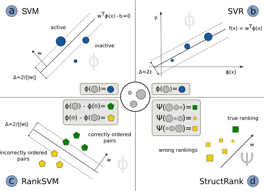
StructRank and other SVM approaches is visualized in Figure 2.2.
For a set x̃ with n molecules, there exist n! possible ways of ranking these molecules. Im-
posing a constraint for each possible ranking would lead to problems becoming too big for
being solved. Therefore, Tsochantaridis et al. [137] proposed a cutting plane approach that
iteratively adds new constraints which violate the current solution. They show that there
exists a polynomially sized subset of constraints whose solution fulfills all constraints of the
full optimization problem. Astonishingly, the optimization problem can be solved efficiently,
an example is the cutting-plane approach used in our implementation of StructRank.
2.2.3 Baseline Models
The novel ranking approach is compared to two algorithms both belonging to the family
of support vector machines: support vector regression (SVR), a state-of-the-art regression
method, often used for virtual screening and ranking SVM (RankSVM), another ranking
approach.
Support Vector Regression (SVR)
Support vector regression [27] is an adaption of classic support vector classifiers for regres-
sion. Like their classification counterpart they follow the Structural Risk Minimization prin-
ciple introduced by Vapnik [138], finding a trade-off between model complexity and training
102.2. Methods
Figure 2.2: Comparison of different support vector machines: a) Support vector machines for
classification learn a linear hyperplane wT φ(x) = b with maximum margin ∆ that optimally
separates active from inactive molecules. b) Support vector regression learns a function
wT φ(x) that predicts binding affinities for each molecule as correct as possible. c) Ranking
SVM generates difference vectors of all possible pairs of molecules. Afterwards similar to
a) a linear hyperplane is learned that separates correctly and incorrectly ordered pairs. d) Ψ
takes a set of molecules x̃ and a ranking p of this set and maps it onto a point in the joint
feature space. StructRank learns a function wT Ψ(x̃, p) which assigns the highest score to the
point representing the true ranking.
11Chapter 2. Ranking Approach to Virtual Screening
error. SVRs learn a linear function f in some chosen kernel feature space [108]. The final pre-
dictor is given by
N
X
f (x) = αi k(xi , x) + b. (2.6)
i=1
The α’s weight the influence of training points xi on the prediction f (x). An -sensitive loss
function is minimized, penalizing only predictions ŷ = f (x) that differ more than from the
true label y:
(
|(y − ŷ)| for |(y − ŷ)| >
`(y, ŷ) = |(y − ŷ)| = (2.7)
0 else.
See Figure 2.2b) for a visualization of SVR. Different studies [24, 74, 150, 67] showed that
SVRs can outperform multiple linear regression and partial least squares and perform on
par with neuronal networks. As implementation LIBSVM together with a Matlab interface
available from http://www.csie.ntu.edu.tw/˜cjlin/libsvm/ (currently in version
3.0, 03.11.2010) is used.
Ranking SVM
As a second baseline we consider a second ranking approach: Ranking SVM [49, 59]. Falling
into the category of pairwise ranking approaches, it maximizes the performance measure
Kendall’s τ . It measures the number of correctly ordered pairs within a ranking of length n,
taking into account all possible n(n−1)
2 pairs. Kendall’s τ has two crucial differences compared
to NDCG: All positions of the ranking have an influence on the final performance unlike for
NDCG, where only the top k positions matter. Additionally all positions have the same
weight, unlike for NDCG, where higher positions are more important. The principle of
Ranking SVM is visualized in Figure 2.2c). In this study the implementation of Chapelle
(available from http://olivier.chapelle.cc/primal/ranksvm.m, accessed on the
03.11.2010) was extended for the use of kernels, according to [19].
2.2.4 Further Approaches and Alternatives
In virtual screening studies a model, generated based on a small number of labeled molecules,
is used to screen large libraries of compounds. These libraries can be considered as unla-
beled data which can be integrated into model generation using semi-supervised learning
approaches. The framework of structured SVMs offers the possibility to integrate semi-
supervised techniques like co-learning [9, 10]. Since this study is directed to the idea of
ranking in virtual screening the aspect of semi-supervised techniques is not discussed and
remains a promising direction of further investigations.
The structure-based ranking SVM with the NDCG loss presented in this work is only one
possible approach to meet the requirements of virtual screening. An alternative approach to
put more emphasis on compounds with a high binding affinity is based on the standard SVR
model and simply re-weights the molecules within the SVR loss function according to their
binding affinity. This leads to a stronger penalization of prediction errors for highly active
molecules compared to molecules offering a low binding affinity. However, experiments
based on this approach led to no performance gain.
122.3. Data
2.3 Data
Sutherland et al. [125] tested spline-fitting together with a genetic algorithm to establish
a good classifier on five virtual screening datasets. Out of these datasets a subset of three
datasets most suitable for regression was selected: The benzodiazepine receptor (BZR), the
enzymes cyclooxygenase-2 (COX-2) and dihydrofolate reductase (DHFR). All datasets were
assembled from literature in order to mimic realistic HTS, i.e. possess high diversity and a
low number of actives. Additionally almost all molecules can be considered drug-like sat-
isfying Lipinski’s rule of five [73]. Compounds with inexact measurements (pIC50 < value
instead of pIC50 = value) which are not suitable for regression approaches were removed
from the original dataset. Table 2.1 summarizes the resulting datasets. A brief description of
the biological function of each target is given below.
Table 2.1: Virtual Screening Datasets
Exact
Endpoint Original Source pIC50 Range
Measurementsa
405 molecules measured by Haefely et al. and
BZR 340 4.27 – 9.47
Cook et al.
COX-2 467 molecules measured by Khanna et al. 414 4–9
DHFR 756 molecules measured by Queener et al. 682 3.03 – 10.45
a
inexact measurements (pIC50 < value instead of pIC50 = value) are excluded from the study
BZR The benzodiazepine receptor (BZR) or GABAA receptor is an ion channel located in
the membrane of various neurons. The opening of BZR induced by its endogenous ligand
GABA causes a membrane hyper polarization which increases the firing threshold. Drugs
like benzodiazepine can bind in addition to GABA in their own allosteric binding site. They
increase the frequency of channel opening thereby amplifying the inhibitory effect of GABA
[118].
COX-2 The enzyme dyclooxygenase 2 (COX-2) together with it’s isoform COX-1 [149]
takes part in the synthesis of prostanoids. While COX-2 is an adaptive enzyme which is
only produced in response to injury or inflammation, COX-1 is a constitutive enzyme which
is produced constantly and provides for a physiological level of prostaglandins [25]. Unspe-
cific COX inhibitors like aspirin produce gastrointestinal side-effects while specific COX-2
inhibitors were shown to reduce gastrointestinal side-effects at the price of increased cardio-
vascular risk [57].
DHFR The enzyme dihydrofolate reductase (DHFR) is involved in the syntheses of purins
(adenine and guanine), pyrimidins (thymine) and some amino acids like glycine. As rapidly
dividing cells like cancer cells need high amounts of thymine for DNA synthesis they are
particularly vulnerable to the inhibition of DHFR. Methotrexat, for example, is a DHFR-
inhibitor which is used in treatment amongst others of childhood leukemia and breast cancer
[7].
2.3.1 Descriptor Generation and Data Preparation
As in previous studies [111, 112] a subset of Dragon blocks (1, 2, 6, 9, 12, 15, 16, 17, 18, and 20
generated by Dragon version 5.5.) is used to represent the molecules. This yielded 728–772
13Chapter 2. Ranking Approach to Virtual Screening
40 40 80
30 30 60
20 20 40
10 10 20
0 0 0
0 1 2 3 0 1 2 3 0 1 2 3
(a) COX-2 (“dense”) (b) BZR (“medium”) (c) DHFR (“sparse”)
Figure 2.3: The distribution of binding coefficients for the virtual screening datasets. The
x-axis shows the binding coefficients (scaled into the range [0,3] for each dataset). The y-axis
shows the number of molecules having that certain binding coefficient. Depending on the
number of molecules with very high binding coefficients we refer to them as “dense” (COX-
2), “medium” (BZR) and “sparse” (DHFR).
descriptors, depending on the dataset. The feature vectors are normalized to zero mean and
unit variance on the training set. In order to keep the results between datasets comparable
the binding coefficients are scaled for each dataset into the range [0, 3] as this is a typical range
when NDCG is used as scoring function for information retrieval datasets [56].
If we examine the distribution of binding coefficients for each dataset (see Figure 2.3), we
can distinguish different types of distributions: For COX-2 we observe a high number of
molecules with high binding coefficients, thus this dataset is called “dense” in the following.
DHFR on the other hand has only a low number number of molecules with high binding
coefficients, thus this dataset is denoted as “sparse”. BZR is in between with few molecules
possessing very high binding coefficients (“medium” ). We will make use of this distinction
later in the result section.
2.3.2 Test Framework
A k-fold cross-validation is implemented to assess performance for the virtual screening
datasets. In order to have similar training set sizes (about 225 molecules), the number of
folds is varied for each dataset: BZR is split into three and COX-2 into two folds. Each
of these folds is once used as test set, whereas the remaining two folds (fold) are used for
training. Then an inner cross-validation with five folds is applied on the training set to
determine the optimal hyperparameters.
For DHFR three folds are employed in the outer cross-validation loop but the single folds are
used for training and the other two form the test set, thus also getting about 225 molecules
in the training set. These cross-validations were performed seven times for DHFR and BZR,
and ten times for COX-2.
As all three approaches share the same underlying SVM framework, they need to determine
the same parameters within the inner cross-validation loop; for the RBF kernel
(xi − xj )T (xi − xj )
k(xi , xj ) = exp − . (2.8)
2dσ 2
the parameters are σ 2 ∈ {0.1, 1, 10} and d given by the number of descriptors. The SVM-
parameter C controlling the model complexity is chosen from the set {0.01, 0.1, 1, 10, 100}.
For the SVR the tube width is varied between {0.01, 0.1, 1}. For the StructRank approach 10,
10 and 30 ranks are considered during optimization.
14Sie können auch lesen