Nexus-e: Integrated Energy Systems Modeling Platform

Federal Department of the Environment,
 Transport, Energy and Communications DETEC
 Swiss Federal Office of Energy SFOE
 Energy Research and Clentech

Swiss Federal Office of Energy SFOE

Final report

Nexus-e: Integrated Energy Systems Modeling
Platform

Cascades Module Documentation

Source: ESC 2019

Date: 27. November 2020

 Location: Bern

 Publisher:
 Swiss Federal Office of Energy SFOE
 Energy Research and Cleantech
 CH-3003 Bern
 www.bfe.admin.ch

 Co-financing:
 -

 Subsidy recipients:
 ETH Zürich
 Reliability & Risk Engineering
 Institute of Energy Technology
 Department of Mechanical and Process Engineering
 Leonhardstrasse 21, 8092 Zürich, Schweiz
 https://rre.ethz.ch/

 Authors:
 Blazhe Gjorgiev, Reliability and Risk Engineering Laboratory, ETH Zürich, gblazhe@ethz.ch
 Giovanni Sansavini, Reliability and Risk Engineering Laboratory, ETH Zürich, sansavig@ethz.ch

 SFOE project coordinators:
 Head of Domain: Yamine Calisesi, yasmine.calisesi@bfe.admin.ch
 Programme Manager: Anne-Kathrin Faust, anne-kathrin.faust@bfe.admin.ch

 SFOE contract number: SI/501460-01

 The authors bear the entire responsibility for the content of this report and for the conclusions
2/25 drawn therefrom.

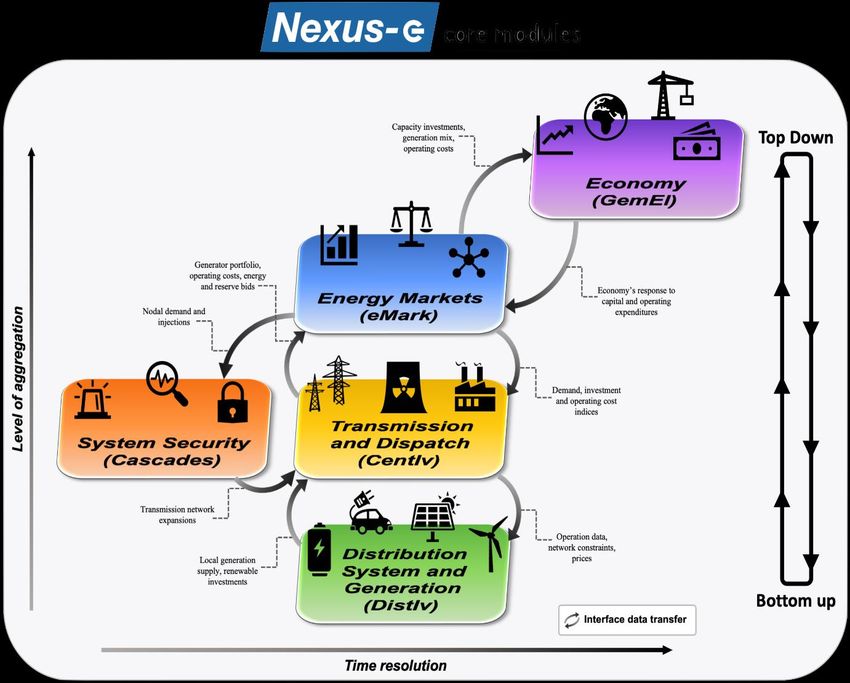
Summary
Policy changes in the energy sector result in wide-ranging implications throughout the entire energy
system and influence all sectors of the economy. Due partly to the high complexity of combining separate
models, few attempts have been undertaken to model the interactions between the components of the
energy-economic system. The Nexus-e Integrated Energy Systems Modeling Platform aims to fill this
gap by providing an interdisciplinary framework of modules that are linked through well-defined
interfaces to holistically analyze and understand the impacts of future developments in the energy
system. This platform combines bottom-up and top-down energy modeling approaches to represent a
much broader scope of the energy-economic system than traditional stand-alone modeling approaches.
 In Phase 1 of this project, the objective is to develop a novel tool for the analysis of the Swiss
electricity system. This study illustrates the capabilities of Nexus-e in answering the crucial questions of
how centralized and distributed flexibility technologies could be deployed in the Swiss electricity system
and how they would impact the traditional operation of the system. The aim of the analysis is not policy
advice, as some critical developments like the European net-zero emissions goal are not yet included
in the scenarios, but rather to illustrate the unique capabilities of the Nexus-e modeling framework. To
answer these questions, consistent technical representations of a wide spectrum of current and novel
energy supply, demand, and storage technologies are needed as well as a thorough economic
evaluation of different investment incentives and the impact investments have on the wider economy.
Moreover, these aspects need to be combined with modeling of the long- and short-term electricity
market structures and electricity networks. This report illustrates the capabilities of the Nexus-e platform.
 The Nexus-e Platform consists of five interlinked modules:
- General Equilibrium Module for Electricity (GemEl): a computable general equilibrium (CGE)
 module of the Swiss economy,
- Centralized Investments Module (CentIv): a grid-constrained generation expansion planning (GEP)
 module considering system flexibility requirements,
- Distributed Investments Module (DistIv): a GEP module of distributed energy resources,
- Electricity Market Module (eMark): a market-based dispatch module for determining generator
 production schedules and electricity market prices,
- Network Security and Expansion Module (Cascades): a power system security assessment and
 transmission system expansion planning module.
 This report provides the description and documentation for the Cascades module, which is utilized
in the Nexus-e framework to assess the security of supply by testing the capability of a power system to
withstand sudden changes, and to provide a transmission system expansion plan if a target level of
security is not satisfied.

 3/25

Zusammenfassung
 Politische Veränderungen im Energiesektor haben weitreichende Auswirkungen auf das gesamte
 Energiesystem und beeinflussen alle Sektoren der Wirtschaft. Aufgrund der hohen Komplexität der
 Energiewirtschaft, wurden bisher nur wenige Versuche unternommen, die Wechselwirkungen zwischen
 den einzelnen Komponenten dieses Systems zu modellieren. Nexus-e, eine Plattform für die
 Modellierung von integrierten Energiesystemen, schliesst diese Lücke und schafft einen interdisziplinäre
 Plattform, in welcher verschiedene Module über klar definierten Schnittstellen miteinander verbunden
 sind. Dadurch können die Auswirkungen zukünftiger Entwicklungen in der Energiewirtschaft
 ganzheitlicher analysiert und verstanden werden. Die Nexus-e Plattform ermöglicht die Kombination von
 „Bottom-Up“ und „Top-Down“ Energiemodellen und ermöglicht es dadurch, einen breiteren Bereich der
 Energiewirtschaft abzubilden als dies bei traditionellen Modellierungsansätzen der Fall ist.
 Phase 1 dieses Projekts zielt darauf ab, ein neuartiges Instrument für die Analyse des
 schweizerischen Elektrizitätssystems zu entwickeln. Um die Möglichkeiten von Nexus-e zu
 veranschaulichen, untersuchen wir die Frage, wie zentrale und dezentrale Flexibilitätstechnologien im
 schweizerischen Elektrizitätssystem eingesetzt werden können und wie sie sich auf den traditionellen
 Betrieb des Energiesystems auswirken würden. Ziel der Analyse ist es nicht Empfehlungen für die Politik
 zu geben, da einige wichtige Entwicklungen wie das Europäische Netto-Null-Emissionsziel noch nicht
 in den Szenarien enthalten sind. Vielmehr möchten wir die einzigartigen Fähigkeiten der
 Modellierungsplattform Nexus-e vorstellen. Um diese Fragen zu beantworten, ist eine konsistente
 technische Darstellungen aktueller und neuartiger Energieversorgungs-, Nachfrage- und
 Speichertechnologien, sowie eine gründliche wirtschaftliche Bewertung der verschiedenen
 Investitionsanreize und der Auswirkungen der Investitionen auf die Gesamtwirtschaft erforderlich.
 Darüber hinaus müssen diese Aspekte mit der Modellierung der lang- und kurzfristigen
 Strommarktstrukturen und Stromnetze kombiniert werden.Dieser Report veranschaulicht die
 Fähigkeiten der Nexus-e Plattform.
 Die Nexus-e Plattform besteht aus fünf miteinander verknüpften Modulen:
 - Allgemeines Gleichgewichtsmodul für Elektrizität (GemEl): ein Modul zur Darstellung des
 allgemeinen Gleichgewichts (CGE) der Schweizer Wirtschaft,
 - Investitionsmodul für zentrale Energiesysteme (CentIv): ein Modul zur Planung des
 netzgebundenen Erzeugungsausbaus (GEP) unter Berücksichtigung der Anforderungen an die
 Systemflexibilität,
 - Investitionsmodul für dezentrale Energiesysteme (DistIv): ein GEP-Modul für dezentrale
 Energieerzeugung,
 - Strommarktmodul (eMark): ein marktorientiertes Dispatch-Modul zur Bestimmung von Generator-
 Produktionsplänen und Strommarktpreisen,
 - Netzsicherheits- und Erweiterungsmodul (Cascades): ein Modul zur Bewertung der Sicherheit des
 Energiesystems und zur Planung der Erweiterung des Übertragungsnetzes.
 Dieser Bericht beinhaltet die Beschreibung und Dokumentation des Cascades-Moduls. Dieses
 Model wird im Rahmen von Nexus-e verwendet, um die Versorgungssicherheit zu bewerten, indem
 die Fähigkeit eines Stromversorgungssystems getestet wird plötzlichen Veränderungen zu
 widerstehen, und um einen Plan für den Ausbau des Übertragungssystems zu erstellen, falls ein
 angestrebtes Sicherheitsniveau nicht erreicht wird.

4/25

Résumé
Les changements de politique dans le secteur de l'énergie ont de vastes répercussions sur l'ensemble
du système énergétique et influencent tous les secteurs de l'économie. En partie à cause de la grande
complexité de la combinaison de modèles séparés, peu de tentatives ont été entreprises pour modéliser
les interactions entre les composantes du système économico-énergétique. La plateforme de
modélisation des systèmes énergétiques intégrés Nexus-e vise à combler cette lacune en fournissant
un cadre interdisciplinaire de modules qui sont reliés par des interfaces bien définies pour analyser et
comprendre de manière holistique l’impact des développements futurs du système énergétique. Cette
plateforme combine des approches de modélisation énergétique ascendante et descendante pour
représenter un champ d'application beaucoup plus large du système économico-énergétique que les
approches de modélisation indépendantes traditionnelles.
 Dans la phase 1 de ce projet, l'objectif est de développer un nouvel outil pour l'analyse du système
électrique suisse. Cette étude sert à illustrer les capabilités de Nexus-e à répondre aux questions
cruciales de comment les technologies de flexibilité centralisées et décentralisées pourraient être
déployées dans le système électrique suisse et comment elles affecteraient le fonctionnement
traditionnel du système. Le but de cette analyse n’est pas d’offrir de conseils politiques, en tant que les
scénarios ne considèrent pas des développements critiques comme l’objectif Européen d’atteindre zéro
émission nette, mais d’illustrer les capabilités uniques de la plateforme Nexus. Pour répondre à ces
questions, des représentations techniques cohérentes d'un large éventail de technologies actuelles et
nouvelles d'approvisionnement, de demande et de stockage d'énergie sont nécessaires, ainsi qu'une
évaluation économique approfondie des différentes incitations à l'investissement et de l'impact des
investissements sur l'économie au sens large. En outre, ces aspects doivent être combinés avec la
modélisation des structures du marché de l'électricité et des réseaux d'électricité à long et à court terme.
Ce rapport illustre les capacités de la plateforme Nexus-e.
 La plateforme Nexus-e se compose de cinq modules interconnectés:
- Module d'équilibre général pour l'électricité (GemEl): un module d'équilibre général calculable
 (EGC) de l'économie suisse,
- Module d'investissements centralisés (CentIv): un module de planification de l'expansion de la
 production (PEP) soumise aux contraintes du réseau, qui tient compte des exigences de flexibilité
 du système,
- Module d'investissements distribués (DistIv): un module PEP de la production décentralisée
 d’énergie,
- Module du marché de l'électricité (eMark): un module de répartition basé sur le marché pour
 déterminer les calendriers de production des producteurs et les prix du marché de l'électricité,
- Module de sécurité et d'expansion du réseau (Cascades): un module d'évaluation de la sécurité du
 système électrique et de planification de l'expansion du système de transmission.
 Ce rapport fournit la description et la documentation du module Cascades, qui est utilisé dans le
cadre de Nexus-e pour évaluer la sécurité de l'approvisionnement en testant la capacité d'un réseau
électrique à résister à des changements soudains, et pour fournir un plan d'expansion du réseau de
transmission si un niveau de sécurité cible n'est pas atteint.

 5/25

Contents
 Summary .................................................................................................................................... 3
 Zusammenfassung ..................................................................................................................... 4
 Résumé ....................................................................................................................................... 5
 Abbreviations ............................................................................................................................. 7
 List of Figures ............................................................................................................................. 7
 List of Tables............................................................................................................................... 7
 1 Introduction ...................................................................................................................... 8
 1.1 Module purpose.............................................................................................................................8
 1.2 Process overview ...........................................................................................................................8
 1.3 Attributes .......................................................................................................................................8
 1.4 Capabilities .....................................................................................................................................8
 1.5 Limitations .....................................................................................................................................9
 1.6 Inputs and outputs .........................................................................................................................9

 2 Related work and contributions .................................................................................... 10
 3 Detailed description of the Cascades module ............................................................... 11
 3.1 Cascading failure simulations model .......................................................................................... 11
 Modeling features ...................................................................................................................................... 11
 Algorithm features ..................................................................................................................................... 14
 3.2 Transmission system expansion planning model ....................................................................... 16
 Modeling features ...................................................................................................................................... 16
 Algorithm features ..................................................................................................................................... 18
 3.3 Cascades simulations options ..................................................................................................... 18

 4 Flexibility ......................................................................................................................... 20
 5 Description of interfaces ................................................................................................ 21
 6 Demonstration of results ............................................................................................... 22
 7 Publications .................................................................................................................... 23
 8 References ...................................................................................................................... 24

6/25

Abbreviations
CCDF complementary cumulative distribution function
DNS demand not served
FCR frequency containment reserve
FD fast decoupled
FRR frequency restoration reserve
GS Gauss-Seidel
IEEE Institute of Electrical and Electronics Engineers
NR Newton-Raphson
OPF optimal power flow
PF power flow
UFLS under-frequency load shedding
UVLS under-voltage load shedding
WECC Western Electricity Coordinating Council

List of Figures
Figure 1. The cascading failure simulation algorithm flow-chart. .......................................................... 12
Figure 2. Expansion planning model flow chart. ................................................................................... 17
Figure 3. An example results of the Cascades module. ....................................................................... 22

List of Tables
Table 1: List of input data. ........................................................................................................................9
Table 2: List of output data. ......................................................................................................................9
Table 3. eMark-Cascades module interface details. ............................................................................. 21
Table 4.Cascades-eMark module interface details. .............................................................................. 21

 7/25

1 Introduction
 1.1 Module purpose
 The purpose of the Cascades module is to: (1) assess the security of supply by testing the capability of
 a power system to withstand sudden changes, i.e. due to component failures; and (2) to provide a
 transmission system expansion plan if a target level of security is not satisfied. The Cascades module
 comprises two models, a cascading failure simulations model and a transmission system expansion
 planning model.

 1.2 Process overview
 The security of supply is assessed with a cascading failure simulations model. The model is initialized
 with sets of contingencies, i.e. potential critical failures that may trigger cascading events. After an initial
 failure is introduced, the model identifies island operations and blackout conditions in the power system.
 Furthermore, the model simulates system automation by performing automatic frequency control to
 restore the power balance in the system by deployment of generation reserves. Moreover, the model
 simulates automatic load shedding in case of system frequency deviations beyond a safety threshold or
 bus voltage magnitudes below a tolerable limit. To calculate the power flows and bus voltages the model
 utilizes an AC power flow algorithm. In addition, the model disconnects transmission elements (lines
 and transformers) due to overloads, i.e. violation of the branch power ratings.
 The transmission expansion planning is performed using a transmission system expansion planning
 model. The model relies on two importance lists, which rank the branches from most important to least
 important with respect to different criteria. Based on the rankings, expansion upgrades are proposed,
 and then each upgrade is assessed using the cascading failure simulation model. The branch upgrade
 providing the best security improvement is added to an expansion list. The process is iteratively repeated
 until a predefined level of security is satisfied or an expansion budget is reached.

 1.3 Attributes
 The following list characterizes some of the main module attributes:
  Deterministic, steady-state model for power system security analysis
  Applies probabilistically selected sets of contingencies (Monte-Carlo approach)
  Evaluates different load and generator conditions at selected time intervals (hours)
  It simulates power system automated responses that react in short time scales (seconds,
 minutes)
  Needs detailed grid and generation unit data
  Uses various solvers for Power Flow and Optimal Power Flow.

 1.4 Capabilities
 The following list describes some of the main capabilities of this module:
  Performs AC and DC cascading failure analyses
  Performs expansion planning using different criteria
 o Target security
 o Available budget
 o Maximum expansions / upgrades
8/25

1.5 Limitations
The following list provides context on some of the main limitations of Cascades:
  The stochastic behavior of the power systems is limited to the initial contingencies
  Transients, e.g. generator swing equations, are neglected
  Voltage control is not considered (under-voltage emergency protection is implemented)
  The expansion planning uses only the existing branches as candidates

1.6 Inputs and outputs
Table 1 and Table 2 list the Cascades module’s required input data and resulting output data,
respectively. It is important to note that the module receives the input data (Table 1) through the eMark-
Cascades interface. However, in a stand-alone run Cascades pulls the data from a dedicated MySQL
database. In this case, the module calculates the generator dispatch and uses the remaining available
capacity as generating reserves. Cascades uses additional input data such as the line failure probability
of branches (lines and transformers), and the under-frequency load shedding (UFLS) and under-voltage
load shedding (UVLS) steps, which are encoded in the algorithm, and described later in this report.
 Table 1: List of input data.

 Variable Resolution Unit Description
 Generator data by unit various Location, capacity, costs, operational parameters, etc.
 Grid topology - various Detailed transmission network data (buses, branches,
 transformers)
 Demand hourly, nodal MW Nodal hourly transmission system demand
 Generator dispatch hourly, nodal MW Generator power injections in each hour
 Reserves hourly, nodal MW Generator power injections in each hour

 Table 2: List of output data.

 Variable Resolution Unit Description
 Branch data - various Expansion plan, i.e. branches to be upgraded
 DNS - - A complementary cumulative distribution function, i.e. risk
 curve
 Outage occurrence - - Transmission system component outage occurrence
 Cascading stages - MW the lines/transformers tripped at each stage and the
 corresponding DNS
 Importance - - Importance/criticality of the transmission system components
 Reserves utilization - MW The what extend each unit is used to provide reserves

 9/25

2 Related work and contributions
 Recent wide-area blackouts such as the 2011 Southwest blackout in Arizona and South California [1]
 and the record-breaking blackout in India [2], suggest that concerns regarding blackout threats in
 transmission systems are well grounded. In response to that, a growing number of analytical and
 simulation methods are emerging for studying the cascading failure in order to prevent and mitigate
 blackouts and improve the reliability of power grids [3]. Herein we provide a review of the most widely
 applied research-grade cascading failure analysis tools [4].
 Hidden Failure (HF) Model
 The HF is a AC PF based model with primary focus on modeling of hidden failures thermal overload and
 generator re-dispatch [5]. The hidden failures of the protection system are modeled by probabilistic
 approaches. Fast simulation technique and heuristic random search are applied to identify the critical
 relays that contribute significantly to the cascades. Maintaining these relays can mitigate cascading
 failures effectively. However, this approach relies heavily on the availability of protection data.
 OPA Model
 OPA model [6] studies the complex dynamics of an upgrading power system with cascading line
 outages. The cascading events are triggered by random line outages, and the line overloads are
 evaluated with DC load flow. The overloaded lines are triggered with a fixed probability. After a line
 outage, the generation and load are re-dispatched using standard linear programming methods with the
 objective of minimizing the load shedding. The distinctive feature of the OPA is that the dynamics of the
 power system upgrade is accounted.
 Manchester
 In the Manchester model [7], a range of cascading failure interactions is presented, which includes the
 cascading tripping of lines, generator instability, under frequency load shedding, post-contingency re-
 dispatch and emergency load shedding for preventing voltage collapse. The model runs an AC PF and
 requires the failure probability of generation and transmission components as well as the probabilities
 of hidden failures as the inputs. The probability of failures can be adjusted according to the effect of
 weather conditions and the model estimates the time required to restore the load following an outage.
 Section 3 of this document presents the details of the Cascades module which encompasses an AC
 based cascading failure simulation model that is similar in concept to the Manchester model.

10/25

3 Detailed description of the Cascades module
Cascades is a system security analysis module comprising: (1) a cascading failure simulations model
and (2) a power system expansion planning model. In the following, both models are described in detail.

3.1 Cascading failure simulations model
The cascading failure model provides insights into the adequacy of the capacity of a transmission
system. The model is characterized by the following functions:
  Simulation of critical scenarios that may trigger a cascading event,
  Identification of island operation within the system,
  Deployment of generation reserves to restore the power balance in the system in case of a
 generation/consumption mismatch or island formation
  Triggering of load shedding due to system frequency deviations beyond a safety threshold/ bus
 voltages magnitudes falling below a tolerable limit
  Identification of blackout conditions in island operation resulting from large power imbalances
 that cause frequency instability
  Computation of the load flow changes across the transmission grid using power flow methods
  Disconnection of overloaded power lines/transformers.

 Modeling features
The cascading failure analysis model procedure is described in the following 12 steps (see Figure 1):

 1. Initial system state
 The initial system state is the starting point of the model. All of the components in the system
 are in service and loads are equal to the forecast. There are no overloads, and the units
 generate power according to a given optimal power flow. In case the dispatch is provided by
 another module/algorithm and results in overloads, Cascades continues the simulations
 considering these overloads, as well.

 2. N-k contingencies
 Here, single or multiple line and transformer contingencies are introduced to initiate sudden
 (unexpected) changes in the transmission system and investigate how the resilience of the
 system is affected by these changes. By default we use a random failure mechanism to initiate
 failures of lines/transformers based on their failure probability. The procedure starts by creating
 a vector of uniformly generated random numbers between 0 and 1. The size of the vector is
 equal to the number of lines and transformers in the system, such that each element in the
 vector corresponds to a particular component. If an element in the generated vector has a value
 equal or smaller than the failure probability of the corresponding component, this component is
 considered failed and added to a contingency list. This procedure is repeated until the
 contingency list has reached a predefined size.
 We use a single probability value for all elements in the system. Due to the low failure
 probability of power system components only a single contingency is found in most runs; double
 or even triple contingencies are sampled only very infrequently. In the end, the contingency list
 consists of a predefined number of sets of contingencies, where each set contains single or
 multiple line or transformer outages.
 The selection of contingencies is executed via Monte-Carlo sampling. Therefore, the larger
 the contingency list the higher the chance of exploring different sets of contingencies and, thus,
 obtaining a more comprehensive evaluation of the system risk. For each set on the contingency
 list a cascading failure simulation is run. After selecting a single set, the related component(s)
 are removed from the system and a new system topology is obtained. 11/25

3. Island identification
 The new topology of the system is checked to see if any islands were created because of the
 contingency. If this is the case, the buses belonging to the respective islands are
 identified.

 Initial system state 1

 2 N-k contingency

 3 Island identification New topology

 i < Nislands

 Detrmine
 4
 frequency, f

 5
 Yes
 UFLS f < 49.5Hz

 6 No

 Restore power balance: Frequency
 i=i+1
 control, Load shedding
 Emergency 9
 automation
 Run AC power flow 7

 Yes
 UVLS Vm< 0.92p.u.
 8
 No
 12 11 10

 Outputs: No Branch flow limits Yes Disconnect
 DNS, outages violation? branch

 Figure 1: The cascading failure simulation algorithm flow-chart.

 4. Check frequency deviation
 The frequency deviation is computed using the following equation [8]:
12/25

− 
 = (1)
 ∑ 1⁄ 

 where is the active power imbalance in MW, represents the set of generators,
 and is the frequency characteristic of th generator (speed droop) in Hz/MW.

5. Emergency automation – frequency
 Emergency under-frequency load shedding (UFLS) schemes are the last measure to be taken
 in order to maintain power system stability after a major disturbance. In principle, whenever the
 frequency deviation is in the allowed range but the available capacities of the synchronized
 generating units are unable to satisfy the load, the UFLS automation uniformly disconnects just
 enough load to reach a new power balance and to avoid a large-scale collapse of the system
 [8].
 The UFLS scheme used in Cascades is based on the Swissgrid transmission code 2013 [9].
 It consists of six steps: if the frequency is smaller than 49.5 Hz, the pumped-storage hydro plant
 operating in pumping regime are disconnected; following are four steps of uniformly
 disconnecting load proportional to the frequency deviation; finally, if the frequency drops for 2.5
 Hz or increases for 1.5 Hz of the nominal, all generators are disconnected.

6. Restore load-generation balance
 As the equation (1) shows, the frequency deviation in the system is proportional to the power
 imbalance. If there is a variation of load demand or island operation in the system, the balance
 between the power generation and load consumption in the system/island may not be
 maintained. The imbalance is measured as the difference between the change of load and the
 change of generation [10, 11]:
 = − (2)

 Restoring the load-generation-balance and, thus, the frequency in the system is performed
 by frequency control actions. When a frequency deviation occurs, all the generators connected
 to the system or the island will ramp up/down to increase/decrease their power output in order
 to compensate for the power imbalance. Generators change the power delivery proportional to
 their ramp rates and are limited by their maximum/minimum operating limits. For the extreme
 case, that there is no load connected to an island, all the generators are shut down. In general,
 generating units reach their new operating points typically in tens of seconds for primary
 frequency control, and in a few minutes for secondary frequency control [12].

7. Power flow calculations
 After restoring the load-generation balance, a power flow study (AC or DC) is performed. In
 case of AC power flow a voltage stability check is performed and the cascading failure
 simulations continue with step 8. In case of DC power flow the cascading failure simulation
 continues directly with step 9, i.e. with an overload check of the transmission system branches.

8. Emergency automation – voltage
 A system may enter a state of voltage instability when it is subject to a disturbance. The steady-
 state threshold is a post-contingency voltage of 92% of the nominal voltage, or 0.92 p.u. [13].
 One of the most economical remedial actions to voltage drop is under-voltage load shedding
 (UVLS) [14]. In order to implement UVLS, the location and magnitude of a voltage drop must
 be identified. In Cascades, under-voltage load shedding is applied to the load directly connected
 to the bus where the voltage violation occurs. In the first step, 25% of the initial load is shed,
 and the voltage magnitude is updated by the AC power flow algorithm. If the voltage violation
 persists, this procedure is repeated until the voltage magnitude is restored back to 0.92 p.u. If
 under-voltage load shedding cannot restore the voltage, the entire load connected to the bus is
 lost.
 13/25

9. Island evaluation
 Steps 4 to 8 are applied to all islands, updating the power flows and bus characteristics of each
 island.

 10. Branch flow limit violation
 After the power flows in each island have been updated, branches with power flows higher than
 their tripping threshold/maximum transmission capacity are identified. Only one line at a time is
 tripped, i.e. the line with the highest overload. The new system topology is returned to Step 3
 for island identification.

 11. Termination criteria
 The simulation is terminated when there are no branch flow violations.

 12. Output results
 Besides the demand not served (DNS) and number of lines/transformers tripped for each set of
 contingencies, the model records the impact of each line/transformer on the DNS, the frequency
 of line/transformer overload, the cascading stages and the corresponding DNS at each stage,
 and the utilization of each unit in positive and negative reserves.

 The procedure from 1 to 12 is repeated for different loading conditions, sampled from a yearly load
 curve. The cascading failure results obtained for each loading condition, are assembled, processed, and
 presented as an output from the model. One of the most important results of the cascading failure model
 is the complementary cumulative distribution function (CCDF) of the DNS. We will refer to it as the
 cascading failure risk curve, or simply risk curve. The risk curve gives the probability of observing DNS
 (blackout intensity) at least as extreme than the one observed.

 Algorithm features
 Cascades incorporates two cascading failure analysis models: the first one relies on DC power flow,
 while the second is AC power flow-based. The preferred choice for solving the AC power flow problem
 is the Newton-Raphson (NR) method; however, the Gauss-Seidel (GS) and Fast Decoupled (FDXB and
 FDBX) methods are also available. The main difference between the two models is that the DC-based
 model does not evaluate bus voltages and, therefore, UVLS cannot be performed. Furthermore, the AC
 model calculates the reactive power flows in the grid, which is not the case with the DC model.
 Consequently, it can be expected that the AC-based model will yield more load shedding events and
 requires more computing time. Both models use MATPOWER package [15] for solving the optimal
 power flow (OPF) and the power flow (PF) problems that are part of the simulations. Furthermore, an
 additional DC-based cascading failure model is available for testing purposes. This model is different
 from the default DC model because it relies on in-built function for the DC power flow calculation and
 MATLAB’s “lineprog.m” for the OPF.
 The cascading failure model can utilizes any of the two available methods for automatic frequency
 control: (1) the default method; and (2) the procured reserves based method. When the default method
 is applied, every available unit is ramped up or down based on the current generation level, and their
 rump rates as described in Section 3.1.6. The procured reserves based method only uses the reserves
 schedule provided by a market/dispatch model. Here the primary and secondary reserves are combined
 and treated as one; this applies to both the positive and the negative reserves. The tertiary reserves are
 activated in case the primary and secondary reserves are not sufficient to balance the load demand. In
 both methods generators are ramped up according to their individual ramp up rates. For the negative
 reserves, besides using the ramp down rates, an additional option is offered where the ramp down is
 performed proportional to the current output of the units. For both frequency control methods, the model
14/25 records the utilization of the reserves from each unit, both positive and negative. These results can later

be used to perform better reserves procurement from a security perspective, i.e. to provide higher
flexibility in the parts of the system where it is mostly needed.
 AC power flow convergence is not always guaranteed and there is a possibility that the algorithm will
fail to obtain solutions under certain conditions. There are various reasons for non-convergence, from
an inadequate initial guess of the bus voltages to voltage collapse. Before any measures are taken we
run simulations using the four available AC PF methods, i.e. NR, FDXB, FDBX, and the GS PF method.
Each of these methods have different convergence properties, thus, the one showing the fewest
convergence issues is selected. When a cascading failure investigation is carried out, it is likely that for
some system configurations the AC power flow will not converge due to the system operating outside
the steady state stability limits. This can be the result of a reduced capacity of the system to transfer the
power from one part to another, or a lack of reactive power to supply load demand, causing a voltage
collapse in some parts of the system. We run a continuation PF to check for system stability limit
violations. To mitigate the convergence problem, a built-in mechanism that can resolve convergence
issues is implemented. The mechanism can take action in four different ways and, depending on the
order in which they are applied, four strategies exist. These actions are: (1) decrease system loading,
i.e. decrease the load and generation simultaneously step-by-step until the AC PF converges; (2)
perform full AC OPF; (3) accept the non-converged solution or consider system blackout; (4) perform
reactive power AC OPF, i.e. fix the active power and run the AC OPF, which results in reactive power
re-dispatch. The preferred (default) order is (1)-(2)-(3), and if (1) is not successful (2) is used and so
forth. Current tests show that in the majority of non-convergence cases action (1) is sufficient; action (3)
is only used in extremely rare situations. When action (3) is used, we accept the non-converged solution
(the default option) and simulate how the cascade progresses. Current tests show that if none of the
above actions is leading to convergence, the non-converged solution is likely to have large
active/reactive power flows in some parts of the system, resulting in overloads. This means that if this
solution is accepted, it is very likely that the cascading will progress further, causing blackouts. However,
the option exists that when action (3) is used a total system collapse is acknowledged, i.e. the algorithm
sheds all load and disconnects all generation. The default value of the load/generator reduction in action
(1) is 5%. Smaller values are not recommended as it may result in longer calculation times, while higher
values may results in unnecessary load shedding.
 In case where the minimum and maximum operational constraints of the slack bus are violated in
the AC PF solution a correction is performed. Namely, the power output is reduced to the maximum
allowed value if the maximum power limit constraint is violated, or increased to the minimum allowed
value if the minimum power limit is violated. The power difference is covered by the reserves or,
alternatively, load shedding is performed. AC power flow studies can result in unrealistic reactive power
flows that, in turn, cause unrealistic power losses. This issue is resolved by ignoring the losses and
treating the power flow as DC. It is worth mentioning that these events are very rare and occur in some
systems more often than in others. The algorithm also has the option to cancel this step.
 The AC-based cascading failure model is adapted to receive generation schedules from a DC-based
dispatch (obtained by a unit commitment / generation scheduling algorithm). The difference between
the AC-based dispatch and the DC-based dispatch is in the power losses occurring in the transmission
lines, which are neglected in the DC approximation. Thus, when a DC dispatch is fed into an AC model,
there will be a power loss mismatch that must be compensated by the slack bus, which may not be the
most economical solution or may even be unfeasible, as the compensation would violate the maximum
power limit constraint of the slack bus. Therefore, a procedure is created that performs a re-dispatch
enabling losses to be distributed to the cheapest generators with available capacity. In the process, all
generators keep the value provided by the DC dispatch except the ones that have to increase their
power output to compensate for the losses. The generators will increase the power output based on the
available capacity such that, if they are scheduled to provide reserves, the reserves are not depleted.
 15/25

However, in case the total amount of additionally available generator power is smaller than the losses,
 the algorithm will use some of the scheduled reserves.
 If the data consists of multiple zones (interconnected power systems, operated independently), the
 algorithm will treat them as one, sharing all available reserves among zones. Future work will upgrade
 the algorithm to perform independent automatic actions within each zone, like secondary frequency
 control and emergency load shedding actions. However, if the neighboring zones of the analyzed zone
 are aggregated, the algorithm offers two options: (1) if there is export reduction into a neighboring zone
 due to events occurring in the zone of interest, add this amount in to the total DNS; (2) only account for
 the events occurring in the analyzed zone, ignoring potential DNS due to export reduction in the
 neighboring zones.
 We use only one failure probability for all lines and transformers in the system, with a default value
 of 0.001. Furthermore, there is the option to use single line rating coefficients (line tripping thresholds)
 for all the lines or multiple ratings for different classes of lines. The purpose of those coefficients is for
 use as tuning parameters when model calibration is performed. When a single line rating coefficient is
 used a single value is set for all lines and transformers in the system. When multiple line rating
 coefficients are used, a unique value is assigned to each component based on the voltage level, i.e. the
 number of coefficients is equal to the number of unique voltage levels. A value of 1, corresponding to
 the nominal line ratings is assigned as the default. The line failure probability and line rating coefficients
 are decision variables in a validation and model calibration procedure we have developed [16]. The
 procedure is based on meta-heuristics with the objective of finding the optimal values for the line failure
 probability and rating, which will enable the simulation results to have the best possible agreement with
 historical data. We have performed this type of model calibration for the Western Electricity Coordinating
 Council (WECC) network, for which historical data on DNS and line outages is available [17, 18].

 3.2 Transmission system expansion planning model
 The objective of the transmission system expansion planning model is to provide an expansion plan that
 achieves a predefined system security. This system security can either be the amount of DNS according
 to historical data or the amount of DNS resulting from simulations of a reference system configuration.
 The selection of the type of system security depends on the availability of historical data for the analyzed
 power system. Herein, the predefined system security will be referred to as the reference security data.
 Furthermore, if a budget for power system expansion is given, the model maximizes the security within
 the given budget. Note that the current model only proposes upgrades of existing branches (parallel line
 or transformer).

 Modeling features
 The transmission system expansion planning model relies on the cascading failure analysis model to
 derive expansion strategies. Two concepts are used: (1) the first concept is based on the impact of
 line/transformer failures on the DNS, which relies on the cascading failure model recording all events
 where an initial contingency results in load shedding. (2) The second concept is based on the frequency
 of line overloads; this concept relies on the cascading failure model recording all line overloads occurring
 after an initial contingency. The model performs the following steps (Figure 2):

 1. Creation of lists
 The impact of line/transformer failures on the DNS, as well as the frequency of line overloads
 are stored in two lists, after which the transmission system lines/transformers are ranked from
 highest to lowest frequency/impact. Additionally, a third list is created as a hybrid of both lists.
 The hybrid list must not have repeating lines/transformers, i.e. if a line/transformer exists in both
16/25 list the one with the highest rank is kept in the hybrid list.

1 2 3 4 No
 Create the Create new
 Asses system
 Importance system difE > 0
 security
 Lists configurations
 Yes

 Cascading failure
 Output the
 simulation model
 needed upgrades
 results

 Figure 2: Expansion planning model flow chart.

2. Expansion strategy

 Each list is used to create an expansion strategy, and each strategy is used to create a
 new/updated network topology. Therefore, three new network configurations are formed. The
 number of lines/transformers to be upgraded from each list is predefined, with the recommended
 number of line/transformer upgrades being equal to one, i.e. only one line/transformer should
 be upgraded in each iteration. This procedure prevents over-investments in the system;
 however, upgrading only one component per iteration can also lead to long computing times.

3. Asses the expansion impact

 After each network configuration has been evaluated separately using the cascading failure
 simulation algorithm, the obtained results are compared. This comparison is based on the
 difference between the simulation results and the (desired) reference system security. One of
 the main results from the cascading failure model is the distribution of DNS events.
 Consequently, we calculate the difference between the simulated and the reference DNS
 distributions. The algorithm has several options for calculating this difference, such as distance
 correlation [19], Kolmogorov-Smirnov test [20, 21], Kullback-Leibler divergence [22], and
 Minkowski distance [23]. The latter is computed as follows:
 1/ (4)
 = (∑| ( ) − ( )| )

 where is a measure of the differences between reference data and simulation results,
 is the complementary cumulative distribution function (CCDF) of the historical
 DNS, is the CCDF of the simulation results, and are the DNS value
 vectors, = 1 results in the Manhattan distance, while = 2 yields the Euclidean distance.
 Because the reference data and the simulation data may not contain the same number of DNS
 values, both vectors are interpolated using linear polynomials to construct new data points within
 a discrete range, thus making the subtraction possible. Equation (4) always results in a positive
 number for both = 1 and = 2. It is, therefore, crucial to know the sign of the function
 difference, which in this case is determined only as the sum of the differences between the
 CCDF of the reference data and the CCDF of the simulation results. A negative sign means that
 the security obtained with the simulations is lower than the security of the system for which the
 reference data is given.
 The function difference (distance) is calculated for all three new system configurations and
 only the system resulting in the highest function difference is kept, the others are discarded. In
 case the required system security is not yet reached, the results obtained from the cascading
 failure simulations of the other two system configurations are used to create the new importance
 lists, which will be further evaluated.
 17/25

4. Stopping criteria
 The function difference is also used as a stopping criteria. In other words the expansion planning
 continues until the function difference becomes a positive value or a predefined number of
 iterations is reached.

 Algorithm features
 The default setting of the transmission system expansion planning algorithm is to calculate and use the
 function difference based on the DNS results. However, the line outage probability function difference
 can be used as an alternative. This difference is calculated as the difference between the line outage
 data (historical or reference system configuration) and the simulation results. One must not confuse the
 failure probability of a line with the line outage probability. The latter is calculated based on the
 participation of each type of outage in the total number of outages. In other words, the number of all
 single component outages is divided by the total number of outages, the number of all double component
 outages is divided by the total number of outages etc.
 Besides the system security, an expansion budget can also be used as the main criterion for the
 expansion plan, enabling the algorithm to find the best expansion plan considering a given budget.
 Violation of the budget is possible. If neither a security criterion nor budget exists, the user is motivated
 to use a maximum number of upgrades.
 The expansion planning algorithm can be executed significantly faster if the user chooses to use only
 one expansion strategy and, thus, only one new system configuration is evaluated at a time. Once the
 expansion method has been applied on a given power system, it becomes evident which expansion
 strategy is giving the best result. Therefore, for further utilization of the algorithm on the same system,
 the user is encouraged to use the strategy that is clearly giving the best results without calculating the
 security impact of the other two strategies. However, if the system is significantly changed the user
 should reassess the expansion strategies and re-select the most adequate one. In case the calculation
 time is not a concern, it is recommended that the user selects the default option, i.e. assessing and
 comparing all strategies.

 3.3 Cascades simulations options
 Besides the possibility of choosing between different cascading failure simulation models and different
 expansion strategies Cascades can be utilized in two modes: (1) stand-alone mode, in which the module
 runs on its own and executes the analyses based on already existing data, and (2) interfaced mode, in
 which Cascades is part of the Nexus-e platform where it exchanges data/results with other modules.
 Furthermore, the user can select the number of demand hours from a yearly demand curve and the
 number of simulations per demand hour. Cascades has the option to select random hours from the load
 demand curve as well as different representative demand hours, e.g. number of peak loads from each
 season, and a combination of peak loads and random hours for each season. As explained in the N-K
 contingencies section, the number of contingencies is randomly selected based on the component
 failure probability. However, the algorithm also has the option to save contingency lists and reload them
 every time Cascades is executed. This option is valuable when one needs to compare the results from
 different cascading failure simulations of the same system and cannot afford to use a large number of
 simulations/contingencies. The number of contingencies and demand hours needed to thoroughly
 explore the system risk depends on the system size. For systems of the order of the 24-bus IEEE test
 system the number of contingencies should be higher than 1000, and the number of demand hours at
 least 18.

18/25

Cascades can be executed in parallel, based either on the contingencies or on the number of
simulation hours. Therefore, the user is encouraged to select one of the parallel execution options, which
will result in smaller computational times. If this option is selected, the algorithm distributes the work
automatically to the available CPU cores or to the number of preselected cores (this setting is available
in the MATLAB parallelization toolbox).

 19/25

4 Flexibility
 The flexibility by Cascades module is captured trough the utilization of available generating reserves. In
 other words, the system frequency changes when the initial failures (contingencies) and the subsequent
 cascading outages result in loss of generator or loss of load in the system. When the frequency deviation
 is within the limits and thus UFLS is not required, the load-generation-balance is restored by frequency
 control, i.e. the power reserves. Therefore, the amount of available and dispatchable (flexible) units and
 their location in the grid will affect system stability and determine if all load will be supplied. In case that
 insufficient generation flexibility exists, the frequency restoration is performed by load shedding. In this
 case, the algorithm records the amount of load shedding as DNS, which is represented with the risk
 curve. Overall, the lack of flexibility in the power system will have a negative effect on the security of
 supply and thus will contribute to the risk of systemic failures, which is captured by the Cascades
 module. Note that the system security is influenced by multiple factors, including the generation mix, the
 share of dispatchable units in the mix, their ramp rates, the location of the units in the grid, the
 transmission capacity, the demand, and the imports/export.

20/25

5 Description of interfaces
The Cascades module is interconnected with the eMark model, i.e. two interfaces are established: 1)
the eMark-Cascades interface, and 2) the Cascades-eMark interface. Through the eMark-Cascades
interface, eMark provides Cascades with the power output of each unit (generation dispatch), the power
exchange between Switzerland and the neighboring countries (imports and exports), and the procured
power reserves (frequency containment reserve (FCR), positive and negative frequency restoration
reserve (FRR)) that each generating unit in the power system provides (see Table 3). The time resolution
of the provided data is one hour and the time horizon is one year. Additionally, eMark passes the power
system physical, the final list of power generation capacities to the Cascades module, and the final
hourly power demand. Note that the reserves procurement provided by eMark are not used in the current
analyses. Instead, all available generators are utilized in providing load-generator balance considering
the generator’s operating limits (ramp rates and minimum/maximum output thresholds) as described in
Section 3.1.6.
 Table 3: eMark-Cascades module interface details.

 Variable Resolution Unit Description
 mpc version - - Version for MatPower mpc structure
 mpc base MVA - MVA Base MVA assumed for MatPower mpc
 mpc bus data by bus various Bus data in MatPower format
 mpc branch data by branch various Line data in MatPower format
 mpc gen data by unit various Generator data in MatPower format
 mpc gen cost data by unit various Generator cost data in MatPower format
 mpc gen info data by unit various Additional generator information
 Load realization hourly, nodal MW Nodal power demand in each hour
 Generation positions hourly, nodal MW Generator power injections in each hour
 FCR procurements hourly, nodal MW Generator power injections in each hour
 Positive FRR procurements hourly, nodal MW Generator power injections in each hour
 Negative FRR procurements hourly, nodal MW Generator power injections in each hour
 Flow type - - The power flow type (AC, DC)
 Swiss zone number - - The Swiss zone number

 The list of branches to be built/upgraded is updated at each iteration between Cascades and eMark,
and the full list is transferred to eMark. In other words, eMark is receiving a list of branches that consists
of the branches from the current iteration and all previous iterations (Table 4). The exchange of
information between the modules continues until Cascades shows no need for further upgrades in the
transmission system, i.e. after the reference security is reached. Furthermore, if there is no significant
improvements to the security over the iterations, although new branches are proposed, the loop is
stopped after a predefined iteration number is reached.
 Table 4: Cascades-eMark module interface details.

 Variable Resolution Unit Description

 mpc branch data (new) - - branches to be upgraded in MatPower format

 21/25