Automatic detection of glasses in ocular images - Hochschule Darmstadt, University of Applied Science - dasec
←
→
Transkription von Seiteninhalten
Wenn Ihr Browser die Seite nicht korrekt rendert, bitte, lesen Sie den Inhalt der Seite unten

Hochschule Darmstadt, University of Applied Science
                    - Fachbereich Informatik -

Automatic detection of glasses in ocular
                            images
         Detection of glasses using 3 different approaches

      Abschlussarbeit zur Erlangung des akademischen Grades
                      Bachelor of Science (B.Sc.)

                            vorgelegt von
                            Florian Struck

        Referent:                 Prof. Dr. Christoph Busch
        Korreferent:              Dr. Christian Rathgeb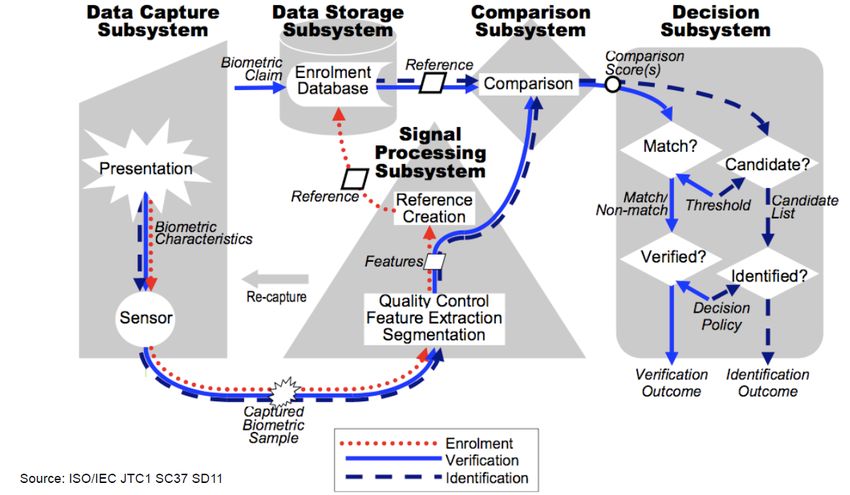
Florian Struck: Automatic detection of glasses in ocular images, Detection of glasses using
3 different approaches, Bachelor of Science (B.Sc.), c July 7, 2017

Supervisors:
Prof. Dr. Christoph Busch
Dr. Christian Rathgeb

Location:
Darmstadt

Time frame:
24.04.2017 - 07.07.2017

                                            ii
Erklärung

Ich versichere hiermit, dass ich die vorliegende Arbeit selbständig verfasst und keine an-
deren als die im Literaturverzeichnis angegebenen Quellen benutzt habe.

Alle Stellen, die wörtlich oder sinngemäß aus veröffentlichten oder noch nicht veröf-
fentlichten Quellen entnommen sind, sind als solche kenntlich gemacht.

Die Zeichnungen oder Abbildungen in dieser Arbeit sind von mir selbst erstellt worden
oder mit einem entsprechenden Quellennachweis versehen.

Diese Arbeit ist in gleicher oder ähnlicher Form noch bei keiner anderen Prüfungsbe-
hörde eingereicht worden.

Darmstadt, 03. Juli 2017

                                            iii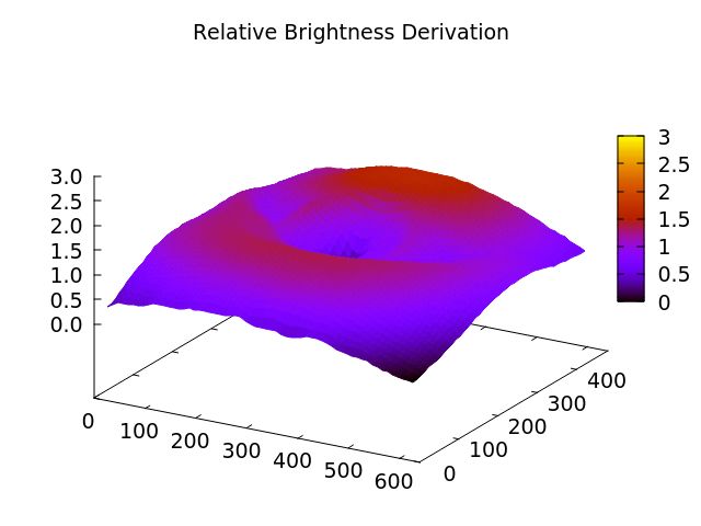
Abstract

In these days there is a large number of deployments for biometric systems. One of the
biggest deployments is the India Aadhaar Identification program with more than 1 billion
registred citizens. In addition there are many border control programs that use biomet-
ric systems for identification. Hence one can suggest that biometric systems become an
integral part of the digital world. Iris is one of the most frequently used biometric charac-
teristic in operational systems because the recoding is convenient and these systems have
a high reliability. Due to the increasing size of the operational deployments of biometric
systems, the requirements in terms of, among others, biometric performance, efficiency
and reliability increase. Especially the large number of glasses wearers is a challenge for
iris recognition systems.

There exist some studies which showed that glasses can deteriorate the biometric perfor-
mance of iris recognition systems, but none of these showed the causes of this deterioration
in detail. We analyzed the influence of glasses on the performance of an iris recognition
system with different experiments and we discovered, that the biometric performance loss
of iris recognition systems correlates strongly with the subjects wearing glasses. A possible
solution to solve this problem is to automatically detect glasses and handle such attempts
separately. We propose 3 approaches to automatic detection of glasses and perform a com-
parative assessment of their accuracy. The proposed approaches are based on: an explicit
algorithmic approach with edge and reflection detection, a deep learning approach and
an approach using filters of binarized statistical image features.

The benchmark that we used was carried out on the CASIA-IrisV4-Thousand database,
which contains 20000 near-infrared eye images; 5336 with and 14664 without glasses. The
explicit algorithm achieved a classification accuracy of 97.18 %, the statistical approach
achieved an accuracy of 98.08 % and the deep learning approach achieved an classification
accuracy of 98.97 %. When using a fusion of all three approaches we were able to classify
99.06 % of images with glasses and 99.71 % of images without glasses. Thereby we were
able to classify 99.54 % of all images on the CASIA-Thousand database in glasses and non-
glasses images. With rejecting the detected glasses on the CASIA-Thousand database, we
increased the iris recognition performance from 9.19 % to 6.61 % EER.

                                             iv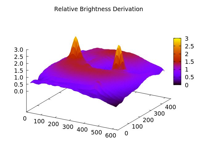
Zusammenfassung

Heutzutage gibt es eine große Anzahl an Anwendungen für biometrische Systeme. Eine
der größten Anwendungen für biometrische Systeme ist das India Aadhaar Identification
Program mit mehr als einer Milliarde registrierter Einwohner. Zusätzlich verwenden aber
auch schon viele Grenzschutz-Programme biometrische Systeme für die Identifizierung.
Daher kann man behaupten, dass biometrische Systeme mittlerweile ein integraler Be-
standteil unserer digitalen Welt sind. Eines der am häufigsten genutzten biometrischen
Merkmale ist die Iris-Textur, da diese komfortable zu erfassen ist und eine hohe Zuver-
lässigkeit aufweist. Durch die steigende Größe von biometrischen Anwendungen steigen
auch die Anforderungen an die biometrische Erkennungsleistung, die Effizienz und Zuver-
lässigkeit. Insbesondere die große Anzahl an Brillenträger ist eine neue Herausforderung
für heutige Iris- Erkennungssysteme.

Es existieren zwar einige Forschungen, die zeigen, dass Brillen die Erkennungsleistung
eines biometrischen Systems verschlechtern können, jedoch wurden die Gründe für diesen
Zusammenhang nicht näher untersucht. Wir untersuchten den Einfluss von Brillen an-
hand verschiedener Experimente und stellten fest, dass es einen starken Zusammenhang
zwischen der Verschlechterung der Erkennungsleistung und der Verwendung von Bril-
lenbilder gibt. Eine Möglichkeit zur Lösung dieses Problems ist, Brillen automatisch zu
erkennen, um diese einer separaten Behandlung unterziehen zu können. Wir testeten drei
unterschiedliche Herangehensweisen für die Erkennung von Brillen und verglichen diese
anhand ihrer Genauigkeit. Zum einen wurde ein expliziter Ansatz mit Kanten- und Re-
flexionserkennung verwendet, zum anderen aber auch ein Deep-Learning Ansatz und eine
statistische Herangehensweise mit Verwendung des BSIF (Binarized Statistical Image Fea-
tures) -Filters.

Für den Benchmark verwendeten wir die CASIA-IrisV4-Thousand Datenbank mit 20000
Bilder (5336 Brillenbilder und 14664 Nicht-Brillenbilder) im Nah-infrarot-Bereich. Der ex-
plizite Algorithmus erzielte eine Genauigkeit von 97,18 %, der statistische Ansatz konnte
98,08 % der Bilder richtig zuordnen und der Deep-Learning Ansatz hatte eine Genauigkeit
von 98,97 %. Durch Fusion aller drei Konzepte waren wir in der Lage, 99.06 % aller Brillen-
bilder und 99.71 % aller Nicht-Brillenbilder richtig zuzuordnen. Auf der CASIA-Thousand
Datenbank konnten wir dadurch 99.54 % aller Bilder erfolgreich klassifizieren. Durch
zurückweisen der erkannten Brillenbilder konnten wir damit die Iris-Erkennungsleistung
auf der CASIA-Datenbank von 9.19 % auf 6.61 % EER verbessern.

                                            v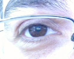
Acknowledgments

First of all, I would like to thank my supervisors Christian Rathgeb and Pawel Droz-
dowski for all the suggestions and assistance during the practice phase and the thesis.
Especiallly, I would like to thank Pawel for the many hours, he corrected my thesis and
assisted with LATEX knowledge.

Further thanks go to my family Susanne, Rolf and Nadine for the support and moti-
vation during my study. Without you, I would not be able to do this study and write this
thesis.

                                           vi
Contents

List of Figures                                                                                ix

List of Tables                                                                                 xi

1 Introduction                                                                                  1
   1.1   Background . . . . . . . . . . . . . . . . . . . . . . . . . . . . . . . . . . .       2
         1.1.1   Biometric system . . . . . . . . . . . . . . . . . . . . . . . . . . . .       2
         1.1.2   Topology . . . . . . . . . . . . . . . . . . . . . . . . . . . . . . . . .     2
         1.1.3   Performance estimation      . . . . . . . . . . . . . . . . . . . . . . . .    4
         1.1.4   Iris signal processing . . . . . . . . . . . . . . . . . . . . . . . . . .     5
   1.2   Motivation . . . . . . . . . . . . . . . . . . . . . . . . . . . . . . . . . . . .     6
         1.2.1   Experiments . . . . . . . . . . . . . . . . . . . . . . . . . . . . . . .      7
   1.3   Research questions . . . . . . . . . . . . . . . . . . . . . . . . . . . . . . . 11

2 Fundamentals                                                                                 12
   2.1   Machine Learning . . . . . . . . . . . . . . . . . . . . . . . . . . . . . . . . 12
         2.1.1   Support Vector Machine . . . . . . . . . . . . . . . . . . . . . . . . 12
         2.1.2   Deep Learning . . . . . . . . . . . . . . . . . . . . . . . . . . . . . . 13
   2.2   Binarized statistical image features . . . . . . . . . . . . . . . . . . . . . . 15

3 Glasses detection                                                                            16
   3.1   Algorithmic feature extraction . . . . . . . . . . . . . . . . . . . . . . . . . 16
         3.1.1   Reflection . . . . . . . . . . . . . . . . . . . . . . . . . . . . . . . . 16
         3.1.2   Edge detection . . . . . . . . . . . . . . . . . . . . . . . . . . . . . 18
         3.1.3   SVM . . . . . . . . . . . . . . . . . . . . . . . . . . . . . . . . . . . 23
   3.2   Deep Learning . . . . . . . . . . . . . . . . . . . . . . . . . . . . . . . . . . 23
         3.2.1   Structure . . . . . . . . . . . . . . . . . . . . . . . . . . . . . . . . 24
         3.2.2   Training . . . . . . . . . . . . . . . . . . . . . . . . . . . . . . . . . 25
   3.3   Binarized statistical image features . . . . . . . . . . . . . . . . . . . . . . 26
         3.3.1   Functionality . . . . . . . . . . . . . . . . . . . . . . . . . . . . . . 26
         3.3.2   SVM . . . . . . . . . . . . . . . . . . . . . . . . . . . . . . . . . . . 27

                                              vii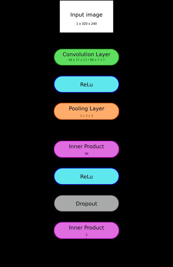
4 Evaluation                                                                               28
  4.1   Procedure . . . . . . . . . . . . . . . . . . . . . . . . . . . . . . . . . . . . 28
  4.2   Results . . . . . . . . . . . . . . . . . . . . . . . . . . . . . . . . . . . . . . 30
  4.3   Fusion . . . . . . . . . . . . . . . . . . . . . . . . . . . . . . . . . . . . . . 30

5 Discussion                                                                               33
  5.1   Error classes . . . . . . . . . . . . . . . . . . . . . . . . . . . . . . . . . . . 33
        5.1.1   Explicit algorithm    . . . . . . . . . . . . . . . . . . . . . . . . . . . 33
        5.1.2   Deep learning . . . . . . . . . . . . . . . . . . . . . . . . . . . . . . 36
        5.1.3   Statistical approach with BSIF . . . . . . . . . . . . . . . . . . . . 37
  5.2   Strengths and weaknesses . . . . . . . . . . . . . . . . . . . . . . . . . . . 39
        5.2.1   Classification accuracy . . . . . . . . . . . . . . . . . . . . . . . . . 39
        5.2.2   Adaptability . . . . . . . . . . . . . . . . . . . . . . . . . . . . . . . 40
        5.2.3   Transparency . . . . . . . . . . . . . . . . . . . . . . . . . . . . . . 41
        5.2.4   Throughput . . . . . . . . . . . . . . . . . . . . . . . . . . . . . . . 43
        5.2.5   Expandability . . . . . . . . . . . . . . . . . . . . . . . . . . . . . . 44
        5.2.6   Summary . . . . . . . . . . . . . . . . . . . . . . . . . . . . . . . . 44

6 Conclusion                                                                               45

Bibliography                                                                                I

                                            viii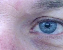
List of Figures

 1.1   General topology of a biometric system [Joi06] . . . . . . . . . . . . . . . .      2
 1.2   Dependence between the False Match Rate, the False Non-Match Rate and
       the used threshold . . . . . . . . . . . . . . . . . . . . . . . . . . . . . . .    4
 1.3   Iris preprocessing steps for feature extraction . . . . . . . . . . . . . . . . .   5
 1.4   Feature extraction from the normalized iris texture to a binary string . . .        5
 1.5   Sample images from the CASIA-Thousand database and the MobBIO database               7
 1.6   Found error classes of failed segmentations . . . . . . . . . . . . . . . . . .     9
 1.7   Quality distribution of all successful segmented images . . . . . . . . . . . 10

 2.1   Example of a 2D SVM Classification, adapted from [Sch16] . . . . . . . . . 13
 2.2   General structure of a deep neuronal network, adapted from [ima] . . . . . 13
 2.3   General structure of a deep convolution network, adapted from [con] . . . . 14
 2.4   Learned BSIF filters [KR12] . . . . . . . . . . . . . . . . . . . . . . . . . . 15

 3.1   Comparison between natural reflections and artificial reflections caused by
       glasses . . . . . . . . . . . . . . . . . . . . . . . . . . . . . . . . . . . . . . 17
 3.2   Visualization of the splitting process . . . . . . . . . . . . . . . . . . . . . 17
 3.3   Visualization of the relative brightness deviation . . . . . . . . . . . . . . . 18
 3.4   Histogram of the reflection score distribution . . . . . . . . . . . . . . . . . 18
 3.5   Visualization of the edge highlighting using a horizontal edge operator . . . 19
 3.6   Applying the calculated threshold for binarization of the grey-value image . 20
 3.7   Dilatation process example . . . . . . . . . . . . . . . . . . . . . . . . . . . 21
 3.9   Visualization of the assignment of the pixels to edges . . . . . . . . . . . . 22
 3.10 Feature score distribution of the explicit algorithm on the CASIA database 23
 3.11 Structure of our deep convolutional network for glasses detection . . . . . . 24
 3.12 Applying the BSIF filter on the input image . . . . . . . . . . . . . . . . . 26
 3.13 Applying the BSIF filter on the input image with glasses . . . . . . . . . . 26

 4.1   Splitting process for cross validation on the CASIA database . . . . . . . . 29

 5.1   Wrongly classified image without glasses due to bad lightning conditions . 34
 5.2   Wrongly classified image without glasses due to bad alignment of the eye . 34
 5.3   Wrongly classified image without glasses due to a strong eyebrows . . . . . 35

                                            ix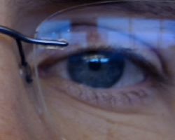
5.4   Wrongly classified image of a glasses due to a strong curvature of the frame
      edges . . . . . . . . . . . . . . . . . . . . . . . . . . . . . . . . . . . . . . . 35
5.5   Wrongly classified image of a glasses due to transparent glasses frames . . . 36
5.6   Error classes of the deep learning approach . . . . . . . . . . . . . . . . . . 36
5.7   Wrongly classified image without classes due to a strong upper eye edge . . 38
5.8   Wrongly classified image with glasses due to a thin glasses frame . . . . . . 38
5.9   Wrongly classified image with classes due to a transparent glasses frame . . 39
5.10 Feature score distribution of the explicit algorithm on the CASIA database 42
5.11 Part of the average histogram from the statistical approach with the BSIF
      filter on the CASIA database . . . . . . . . . . . . . . . . . . . . . . . . . 42
5.12 Learned convolution filter in our glasses identification network . . . . . . . 43

                                           x
List of Tables
1.1 Iris recognition performance on our base experiment . . . . . . . . . . . . . 8
1.2 Statistics of the OSIRIS segmentation performance . . . . . . . . . . . . . 8
1.3 Iris recognition performance on successfully segmented images . . . . . . . 9
1.4 Iris recognition performance on successful segmented images and usage of
masks and a threshold of 0.60 . . . . . . . . . . . . . . . . . . . . . . . . . 10
3.1 Example list of measured edges . . . . . . . . . . . . . . . . . . . . . . . . 22
4.1 The characteristics of the CASIA database . . . . . . . . . . . . . . . . . . 28
4.2 Results of the evaluation on the CASIA database . . . . . . . . . . . . . . 30
4.3 Results of the AND fusion on the CASIA database . . . . . . . . . . . . . 30
4.4 Results of the OR fusion on the CASIA database . . . . . . . . . . . . . . 31
5.1 Summary of the strengths and weaknesses of the proposed approaches . . . 44
xiAcronyms
FMR False match rate
FNMR False non-match rate
EER Equal Error Rate
NIR near-infrared
SVM Support Vector Machine
DNN Deep Neuronal Network
CNN Convolution Neural Network
BSIF binarized statistical image features
xiiChapter 1
Introduction
Due to growing networking and digitalisation, reliable, efficient and user-friendly authen-
tication of users becomes more and more important. Besides traditionally authentication
methods that are based on either knowledge (e.g. passwords) or on possession (e.g. to-
kens, access cards), biometrics has arisen as an increasingly viable alternative. Biometric
systems make it possible to identify users using biological and behavioural features of an
individual [Joi12]. In contrast to knowledge or physical tokens biometric features cannot
be forgotten, lost or passed on to another person. This makes it a comfortable and secure
way to authenticate users.
One of the most popular biometric characteristics is the iris texture. One reason for
this is that the iris can be recorded comfortable because the eye is an externally visible
organ. Further the iris has a high collectability and permanence [JBP06] so that it can
be used for a fast and reliable biometric system. An important factor for the biometric
performance of a biometric recognition system is the quality of the captured sample. The
better the sample quality the better the biometric recognition performance. For iris recog-
nition it is important that the eye is opened widely and the iris texture is clearly visible
and unoccluded. Besides natural noise factors such as eyelids or eyelashes, which cannot
be prevented, there are environmental factors that can further deteriorate the quality of
a sample [Joi15]. Since many of todays biometric systems are unsupervised, there is no
human who controls the capturing process, these factors have to check automatically by
the biometric system. One of these factores is the wearing of glasses during the captur-
ing process. In contrast to many other environmental factors (e.g. lighting, reflections)
that can already be detected automatically, the detection of glasses is more complex and
needs greater attention. Therefore we tried to detect glasses on eye images automatically,
so that an iris recognition system would be able to handle them separately to achieve a
better biometric performance. For this purpose we tried 3 different methods for glasses
detection. The first approach was an explicit algorithm that calculates 2 metrics that
describe the edges and reflections on an input image and uses a Support Vector Machine
1(SVM) to classifiy the images with the calculated metrics. The second approach that we
have tested uses a deep convolution network for direct classification. As third method, we
used a statistical approach that creates a histogram of an input image using the BSIF
filter and uses a SVM for classification. After we tested the approaches on their own we
merged the decisions with different rules to get better results.
1.1 Background
In order to understand the experiments that we have done to investigate the influence of
glasses on iris recognition systems, we give a short introduction about biometric systems
and techniques to estimate their performance.
1.1.1 Biometric system
A biometric system is used to identify or verify an individual based on its biometric
features. It uses the distinguishable biological or behavioural characteristics to recognize
a registered user of a system. For this it saves the biometric characteristics of an individual
in a database so that it is able to compare the characteristics with other samples.
1.1.2 Topology
The general topology of a biometric system can be seen in figure 1.1.
Figure 1.1: General topology of a biometric system [Joi06]
2In the following part, the subsystems of a general biometric system are explained. The
used biometric terms are defined in ISO/IEC 2382-37 [Joi12].
Data Capture Subsystem This subsystem has the tasks to capture the biometric fea-
tures from a user into a biometric sample. This is done by sensors which record the needed
characteristics. In the case of iris recognition these sensors are generally cameras that take
pictures of the eyes.
Signal Processing Subsystem This subsystem processes the captured sample of the
Data Capture Subsystem. For this it runs multiple steps such as quality control, feature
extraction and segmentation to create a reference. While the enrolment process the ref-
erence is given directly to the Data Storage System, where it will be saved in a database.
Otherwise the reference goes to the Comparison Subsystem.
Data Storage Subsystem While running an enrolment process, this subsystem saves
the enrolled reference in the database, so that is can be loaded later for verification or
identification. For verification, it loads the reference of the user based on an identity claim
and sends it to the Comparison Subsystem. When running an identification process, it
loads all references from the database and sends them to the Comparison Subsystem.
Comparison Subsystem In this subsystem, the captured sample from the Signal Pro-
cessing Subsystem and a saved reference from the Data Storage System are compared.
As a result of the comparison, one or more comparison scores are generated that indicate
how similar or dissimilar the two samples were. These scores are sent to the Decision
Subsystem.
Decision Subsystem This is the last subsystem and runs in two different modes: ver-
ification and identification. In the verification mode, the system decides on the basis of
a single comparison score from the Comparison Subsystem and an associated threshold
whether there is a match or not. If there is a match, the person whose characteristic was
captured in the Data Capture Subsystem is verified successfully, otherwise the verifica-
tion fails. In the identification mode, this subsystem receives a list of comparison scores
from the Comparison Subsystem. With the aid of the best score or an additional decision
logic, the system decides with thresholds whether there is a candidate or not. If there is
a candidate, the associated identity according to the database will be outputted, else the
identification fails.
31.1.3 Performance estimation
For comparing and benchmarking the performance of a biometric system, there are dif-
ferent metrics which are standardized in ISO/IEC 19795-2 [Joi07]. Two of these are the
False Match Rate (FMR) and the False Non-Match Rate (FNMR).
False Match Rate (FMR) This metric indicates the proportion of impostor attempts
that were accepted falsely. It depends on the used decision threshold. For dissimilarity
scores, the higher the threshold the higher is the False Match Rate.
False Non-Match Rate (FNMR) This metric indicates the proportion of genuine
attempts that were rejected falsely. Like the False Match Rate it depends on the used
decision threshold. For dissimilarity scores, the higher the decision threshold, the lower
the False Match Rate.
Equal Error Rate (EER) This metric indicates the point were the False Match Rate
and the False Non-Match Rate are equal. It means that there is the same proportion
of impostor attempts that were accepted falsely, as genuine attempts that were rejected
falsely. This is a common, one-number metric to evaluate the performance of a biometric
system.
The dependence between the FMR, FNMR and the used threshold can be seen in fig-
ure 1.2.
Figure 1.2: Dependence between the False Match Rate, the False Non-Match Rate and
the used threshold
41.1.4 Iris signal processing
The signal processing in a iris recognition system can be distinguished into segmenta-
tion/normalization and feature extraction. The described processes are used in essentially
all operational iris deployments.
Segmentation/Normalization
In this step, an algorithm locates the outline of the iris (visualized in figure 1.3b) and
normalizes it into a rectangular area (figure 1.3c) of a constant size according to Daug-
man’s rubber sheet model [Dau04]. In addition it can generate a noise mask (figure 1.3d)
of parts that do not belong to the iris texture such as eyelids or eyelashes. This prevents
that the feature extraction algorithm processes areas that do not contain iris feature,
and thereby deteriorate the recognition performance. This preprocessing ensures that the
feature extraction algorithm has an input of a constant size and can extract the features
independent of the iris position and pupil dilation.
(a) Original photo (b) Segmented image
(c) Normalized iris texture (d) Mask for the normalized iris texture
Figure 1.3: Iris preprocessing steps for feature extraction
Feature extraction
After creating a normalized texture with an optional noise mask, a feature extraction
algorithm transforms it into a binary template of a constant size (called iris code).
FE algorithm
GGGGGGGGGGGGGGGGGGA 001100101110101110010000...
Figure 1.4: Feature extraction from the normalized iris texture to a binary string
As J. Daugman [Dau04] already introduced, the comparison of two binary iris templates
5can be done by calculating the Hamming distance. The formula for the calculation of the
dissimilarity scores of two binary iris templates can be expressed as
k(codeA ⊕ codeB) ∩ maskA ∩ maskBk
hd = (1.1)
kmaskA ∩ maskBk
where codeA is the bit vector of the first template, codeB is the bit vector of the second
template, maskA is the bit vector of the mask of the first template and maskB is the bit
vector for the mask of the second template.
1.2 Motivation
With increasing number of use cases for biometric systems, the systems have to become
more robust against different environmental influences which can deteriorate the quality
of the captured samples. While earlier most biometric systems were permanently installed
with consistently good lightning conditions, more and more of today’s biometric systems
are based on mobile hardware, such as mobile iris sensors or smartphones , operating
under unconstrained and unsupervised environments. In addition, while earlier only in-
structed persons used these relatively small systems, today’s large-scale biometric systems
are used by the general public, who do not always know how to use such systems cor-
rectly. A wrong usage of the sensors during the capturing process can result in a bad
sample quality and as H. Proença and L. Alexandre [PA05] have already showed, leads to
a worse segmentation performance. That is why automatic sample quality control must
be performed by a biometric system, in order to ensure correct operation.
There are many quality metrics defined in the ISO/IEC 29794-6 [Joi15] to measure the
quality of iris samples. The task for a biometric system is to calculate those quality metrics
for a captured sample automatically to decide if the quality is sufficient. Such an auto-
matic quality estimation was done, for example, by Kalka et al. [KZSC10] who developed
an automatic method to estimate the quality of iris samples.
Besides the general sample quality, there is an additional factor. Many people have to
wear glasses. For example, in Germany, almost two thirds (63.5 %) of the population
which age is over 15 are glasses wearers [fDA15]. The number of glasses wearers between
20- and 29 is increasing noticeably. As Lim et al. [LLBK01] has already investigated, the
usage of samples with glasses deteriorate the preprocessing performance and therefore the
overall performance of an iris recognition system. However, the causes for this deteriora-
tion were analyzed rarely by the authors so that we investigated the underlying causes of
this quality deterioration in greater detail.
61.2.1 Experiments
To investigate the influence of glasses under different basis conditions, we used both near-
infrared (NIR) and visible wavelength (VW) images of the CASIAv4 thousand database
[Chi], thereby yielding more general and comprehensive results. We manually categorized
the images in two classes: images with glasses and images without glasses, thus we were
able to evaluate the recognition performance of these classes separately. Then we seg-
mented all images using the OSIRIS [ODGS16] tool, extracted their features using the
LogGabor implementation of the USITv2-Toolkit [RUWH16] and saved the references
sorted by the subject id. After that we were able to calculate the genuine and impostor
scores for both classes by applying the commonly used, Hamming distance based, com-
parator. At the end of each experiment, we calculated the Equal Error Rate (EER) on the
basis of the calculated scores, so that we were able to assess the recognition performance.
In figure 1.5 you can see sample images from the databases that we used in our ex-
periments. Image 1.5a-d is from the MoBIO database, image 1.5e-h is from the CASIA-
Thousand database.
(a) (b) (c) (d)
(e) (f) (g) (h)
Figure 1.5: Sample images from the CASIA-Thousand database and the MobBIO database
7Baseline
At the beginning of our research, we started with a baseline evaluation of the categorized
databases. The results are shown in table 1.1. As you can see, using samples with glasses
leads to a strong deterioration of the iris recognition performance on both databases.
Further analysis showed that there were many high genuine comparison scores on samples
of glasses, which causes a higher EER.
Glasses No glasses
Database Genuine Impostor EER Genuine Impostor EER
comp. comp. comp. comp.
CASIA 10338 999000 12.16 % 52278 999000 6.86 %
MobBIO 658 10712 40.04 % 4020 10712 35.26 %
Table 1.1: Iris recognition performance on our base experiment
Segmentation evaluation
Next, we evaluated the segmentation performance by visually inspecting the segmented
images for correctness. In table 1.2 you can see the statistics of the OSIRIS segmentation
performance on the used databases.
Glasses No glasses
Database Successful Failed segm. Quota Successful Failed segm. Quota
segm. segm.
CASIA 5105 231 95.67 % 14031 633 95.68 %
MobBIO 127 136 48.29 % 842 535 61.15 %
Table 1.2: Statistics of the OSIRIS segmentation performance
While on the MobBIO database the quota of the successful segmentations on images
with glasses was much worse than on images without glasses, on the CASIA-Thousand
database the proportions were almost equal. This shows that on the CASIA-Thousand
database glasses have significantly less influence on the segmentation performance than
they have on the MobBIO database. One reason for the small difference could be that
glasses have less influence on the photo quality when using near-infrared light instead of
visible light.
8We analyzed the wrongly segmented samples and found 4 error glasses, which are shown
in figure 1.6.
(a) (b)
(c) (d)
Figure 1.6: Found error classes of failed segmentations
As you can see 3 of 4 error classes were caused by glasses, whereas the most common error
class (figure 1.6a) was independent of glasses. After sorting out all failed segmentations,
we repeated the evaluation. The results can be seen in table 1.3.
Glasses No glasses
Database Genuine Impostor EER Genuine Impostor EER
comp. comp. comp. comp.
CASIA 9729 998001 10.67 % 48744 998001 3.79 %
MobBIO 263 9037 27.92 % 2264 9037 28.91 %
Table 1.3: Iris recognition performance on successfully segmented images
The removal of false segmentation has lead to a significantly better performance on both
classes. However, on samples without glasses the performance is still better than on sam-
ples with glasses. We think that the EER of 27.92 % on the MobBIO database is a
measuring error because, this is the only exception where the performance on samples
with glasses is better than the performance on samples without glasses. All other calcula-
tions show consistent results. One possible reason for this measuring error could be that
there were only few genuine comparisons (263).
9Quality evaluation
In the last experiment we analyzed the quality of the samples using the Usable iris area,
which is a general metric for quality estimation of iris images and is standardized in ISO
29794-6 [Joi15]. At first, we plotted the quality distribution of both databases, which can
be seen in figure 1.7.
Iris Area Distribution Iris Area Distribution
1 1
glasses glasses
no glasses no glasses
0.8 0.8
Ratio Accepted Images
Ratio Accepted Images
0.6 0.6
0.4 0.4
0.2 0.2
0 0
0 10 20 30 40 50 60 70 80 90 100 0 10 20 30 40 50 60 70 80 90 100
Iris Area (%) Iris Area (%)
(a) Distribution of the usable iris area (b) Distribution of the usable iris area
on the CASIA-Thousand database on the MobBIO database
Figure 1.7: Quality distribution of all successful segmented images
The diagram shows that samples with glasses have a consistently smaller visible iris area
than samples without glasses. After getting an impression of the quality distribution, we
decided to exclude some of the images with small visible iris area. For our evaluation
we used the threshold 0.60. This threshold rejects the poorest images and nevertheless
accepts the majority of images with a better quality. The results are shown in table 1.4.
Glasses No glasses
Database Genuine Imposter EER Genuine Imposter EER
comp. comp. comp. comp.
CASIA 6366 935145 7.83 % 36573 935145 2.50 %
MobBIO 194 8572 26.06 % 1803 8572 25.11 %
Table 1.4: Iris recognition performance on successful segmented images and usage of masks
and a threshold of 0.60
Although we sorted out all images with a small usable iris area, the performance difference
between samples of glasses and samples without glasses kept significantly. This means that
even in systems with high quality requirements, there can be a strong deterioration of the
iris recognition performance when accepting samples with glasses.
10Conclusion
During the experiments, we found multiple causes for the deterioration of the iris recogn-
tion performance when using samples with glasses. In our base experiment, we showed
that even if the overall iris recognition performance is relatively bad, glasses have a great
negative impact on the performance. After analyzing the segmentation performance, we
found out that the most types of unsuccessful segmentations occurred only on images of
glasses even, though the most common type of segmentation error occurred independently
of glasses. It turned out that the influence of glasses on the segmentation performance
depends on the used wavelength. While on the NIR photos of the MobBIO database
there was a significant difference, on the VW photos of the CASIA database the error
rates were almost equal. The calculation and visualization of the usable iris area of the
samples showed that images without glasses had a consistently greater area. In addition,
we demonstrated that even higher quality control thresholds do not change the fact that
images with glasses have a worse performance on iris recognition systems than images
without glasses. Overall, we can say that glasses consistently deteriorate the performance
of iris recognition systems and should be handled separately. In order to do so, there has
to be an automatic method of glasses detection on input samples.
1.3 Research questions
In this thesis, we develop different approaches for glasses detection and benchmark them
against each other. The goal of this research was to answer following questions:
1. Which approaches are suitable for detecting glasses? How do they work?
2. Where are their strengths and weaknesses? How can weaknesses be avoided and
strengths be used better?
3. How well do they complete each other? Is it possible to offset weaknesses of one
approach by adding a second approach? How well does the fusion of all different
approaches perform?
11Chapter 2
Fundamentals
In the following chapter we describe fundamental concepts that we used in the experiments
for the thesis. In addition we mention machine learning approaches and the BSIF filter.
2.1 Machine Learning
Machine Learning makes it possible to recognize relationships in datasets automatically.
Therefore, it is a popular technique to handle complex data. Machine Learning can be
divided into several approaches, which differ in the way their algorithm handle the data.
In this thesis, we only used supervised learning which is commonly used for automatic
classification. The usage of machine learning can be distinguished into a training phase
and a prediction phase. In the training phase, the algorithm reads input data and its
associated output data and learns the relationships between these datasets. By definition
of supervised learning, the input data of the training set has to be labeled [sup]. This
means that a groundtruth set for the training data has to be created which contains the
expected associations. In the prediction phase, the algorithm reads only input data which
is unknown to the algorithm and process it based on the previously learned relationships.
2.1.1 Support Vector Machine
A Support Vector Machine (SVM) is a supervised machine learning approach to classify
input vectors into two categories. The basic operating principle of classification can be
seen in figure 2.1.
During training the SVM reads multiple vectors that are represented as points in a hy-
perspace, whereby each point pertains to specific category. It tries to create a hyperplane
between the points of the different categories, so that the groups of points are separated
clearly. For each training iteration the SVM tries to enhance the distance between the
hyperplane and the points to optimize the classification performance [Chr04]. This has
the advantage that even if there are new points that are lying closer to the points of the
12Figure 2.1: Example of a 2D SVM Classification, adapted from [Sch16]
other category the separation still works. For the optimization process only the so-called
support vectors, which are points that are lying closely to the other category (outlined
points in figure 2.1), matter.
In the prediction phase the SVM gets an input vector and decides on the basis of the
position of the associated point in the hyperspace the category to which it belongs. These
relatively simple calculations allow it to categorize complex data in a short time.
2.1.2 Deep Learning
Deep Learning describes combination of multiple neuronal layers that are connected to
each other. Each of those learns particular connections of the previous layer and passes
them to the next layer. This allows to learn very complex relationships for doing costly
processing steps. The basic structure of a deep neuronal net (DNN) can be seen in figure
2.2.
Figure 2.2: General structure of a deep neuronal network, adapted from [ima]
13It contains an input layer, multiple hidden layers and an output layer. Each layer con-
tains several neurons that are derived on the biological neurons of the human brain. For
communication the neurons are connected to each other whereby each connection has a
weight. Like the biological neurons, the artificial neurons have an activation threshold for
the sum of the incoming signals. Once this threshold is exceeded the triggered neuron
sends a signal to the following neurons.
During the training phase, the source data is given to the input neurons that sends the
calculated signals to the next layer. At the end of the neuronal net the output is compared
to the expected output of the training data. By using backpropagation [bac], the weights
are adjusted so that the output of the net approximates the expected output.
In prediction mode, the input data is directly transformed into the output data by using
the learned weights.
Deep Convolutional Network
A convolutional neuronal network [con] is a subset of a neuronal net. In contrast to the
neuronal network that uses neurons, a convolutional network contains several filters per
layer. Convolutional networks that have many layers are also called deep convolutional
networks. This type of neuronal network is particularly very suitable for image processing,
because it is able to recognize patterns in images efficiently. The common structure of a
deep convolutional network for image processing can be seen in figure 2.3.
Figure 2.3: General structure of a deep convolution network, adapted from [con]
At the beginning of such a network, there are multiple combinations of convolution and
pooling layers. These layers extract the features from the input image. While convolution
filters learn known patterns from the input matrix, pooling layers scale down the size of
the input, which enhance the calculation performance. At the end of the feature extraction
part there is a set of fully connected neurons, which are responsible for the assignment
of the extracted features into classes. The more difficult the processing task of the input
image the more extensive has to be the network structure.
14In summary it can be said that deep learning approaches are very powerful to solve clas-
sification problems which is why we used it for our experiments. However, the mentioned
parts are only a small extract of the broad and complex subject area of machine learning.
2.2 Binarized statistical image features
In order to recognize image patterns and process images, local image descriptors in form
of filters are commonly used. They are able to map local brightness curves into scalar val-
ues, which represent the local structure of an image part. A filter consists of a matrix of a
fixed size, which contains weights for mapping the pixel values to the final filter response.
Commonly, the filter is applied on all pixels of an image to create a detailed overview of
the brightness features of an image. In this section, we introduce the Binarized Statistical
Image Features (BSIF) filters.
The BSIF filter was first presented by J. Kannala and E. Rahtu in [KR12]. In contrast to
the most filters, which use fixed weights, the weights of the BSIF filters are determined by
training on natural images. Figure 2.4 shows an example of pre-learned 9x9 pixels BSIF
filters.
Figure 2.4: Learned BSIF filters [KR12]
The BSIF filter consists of several independent subfilters. Each subfilter has its own
weights and therefore produces its own response. The response is binarized by its sign.
As final filter response, the output bits of the different subfilters are appended and the
results is interpreted as a decimal number. Therefore, the final filter response depends on
the training data of the subfilters, their size and the number of filters that were used for
the final response. Commonly, the filter response is transformed into a histrogram of the
length l = 2n where n is the number of subfilters which were used. For the experiments in
this thesis, we used the pre-learned filters and matlab implementation from J. Kannala
[bsi].
15Chapter 3
Glasses detection
In this chapter, we present 3 different automatic approaches for glasses detection in ocular
images. All approaches uses completely different stategies to select and extract features
from the images and use them for classification.
3.1 Algorithmic feature extraction
This approach is based on an explicit algorithm, that analyzed fixed features on images
with glasses to generate metrics which can be used for classification. The procedure of
this algorithm is inspired by how a human might perceive glasses. We analyzed multiple
images to find features that are suitable for detecting glasses. These features had to be
extracted easily by an machine algorithm and had to be robust against environmental
factors such as fluctuations in illumination. In our implementation we used the OpenCV
[Ope17] library for the image processing and uses auxiliary functions of the Boost [Boo17]
library.
3.1.1 Reflection
The first feature that we have considered as suitable was the strong reflection on many
glasses. As you can see in figure 3.2a, the natural reflections on images without glasses are
much smaller than the reflections in figure 3.2b, which shows an image with glasses. This
makes it easy to distinguish between natural reflections and artificial reflections which are
caused by glasses.
16(a) Image without glasses (b) Image with glasses
Figure 3.1: Comparison between natural reflections and artificial reflections caused by
glasses
For the reflection detection we split the image into overlapping blocks of a fixed length.
These blocks had to be big enough to ignore small natural reflections, but small enough
to highlight bigger reflections which are caused by the glasses. On the CASIA database
we used a block size of 30x30 pixels. In order that the blocks cover the reflection areas as
well as possible we shifted the blocks by one-third of the block size which resulted in 10
pixels. In figure 3.2 you can see an example how the image is divided into blocks where
the alignments for the blocks are marked green and the relevant blocks are marked red.
(a) Image without glasses (b) Image with glasses
Figure 3.2: Visualization of the splitting process
The measuring of the brightness of each block was done by calculating the average grey
value of the block and divided it by the average grey value of the complete picture. The
usage of relative brightness scores instead of the average pixel value in a block makes it
more robust against fluctuations in illumination. For instance, when an image is overex-
posed, the bright areas must not be identified as reflections. Since the average grey value
of such images is relatively high, bright blocks lead to a significant lower reflection score
than on images with a better exposure. At the end of this step we get a 2-D map of
relative brightness deviation. The visualization of this map can be seen in figure 3.3.
17(a) Image without glasses (b) Image with glasses
Figure 3.3: Visualization of the relative brightness deviation
The big reflections lead to high relative brightness scores whereas small reflections have
very little influence on the scores. For the final score, only the highest brightness score is
considered. This final score can be used for classification either with a specific threshold or
with a machine learning approach such as SVM. The distribution of the reflection scores
on the CASIA database can be seen in figure 3.4. In our first version with a fixed relative
brightness threshold, a threshold of 2.0 turned out as suitable.
Reflection score distribution
0.12
Glasses
0.1 No glasses
0.08 t = 2.0
Frequency
0.06
0.04
0.02
0
1.4 1.6 1.8 2 2.2 2.4 2.6 2.8 3 3.2
Reflection score
Figure 3.4: Histogram of the reflection score distribution
3.1.2 Edge detection
After we were able to measure strong reflections and used it for glasses classification, we
searched for further features because not all glasses cause reflections. The next feature that
we considered as useful were the edges of the glasses frame. In contrast to the natural
small edges on the eye, these frame edges are more pronounced and longer. However,
the measuring of these edges is more complex than the measuring of the reflection. In
contrast to the human brain that can detect edges very easly, the edge detection on
computer is significantly harder. Therefore, we split the edge measuring algorithm into
several processing steps. The first 3 steps enhance the edges, so that the last 3 steps are
able to measure them.
18Edge enhancement
In the first step, we deliberate how to highlight the important frame edges while ignoring
small natural edges of the eye. Therefore we analyzed the differences between the 2 classes
of edges. While the natural edges are mostly short and have no specific direction, the
frame edges are significantly longer and run commonly horizontally as long as the eye is
aligned properly. The edge detection is commonly done by specific convolution matrices
that measure the brightness gradient of a part of an image. One of the most popular
edge detection operator is the Laplacian Operator, which is able to detect edges of both
horizontal direction and vertical direction. As mentioned above, we only want to detect
horizontal edges which is why we used another more simple edge detection operator, which
can be seen in figure 3.5b. After applying the operator on the input image 3.5a, we obtain
an image of the detected edges which is shown in figure 3.5c. Since these convolution
matrices do only calculate the local brightness gradient, the output image is independent
of the average brightness of the input image.
0 0 0
0 -1 0
0 1 0
(a) Original image (b) Simple horizontal (c) Image after edge operator1
edge detection operator
Figure 3.5: Visualization of the edge highlighting using a horizontal edge operator
The result of this process step is grayscaled image with a average pixel value of 127.
Edge binarization
In the next step, we transformed the grayscaled image into a black and white image by
applying a relative threshold. Thereby, we ignore blurred edges and brightness transitions
from dark to light. This means we accept only sharp brightness transitions from light to
dark, mostly the bottom edge of a glasses frame.
The absolute threshold is selected, so that only a specified percentage of the brightest
pixels is accepted. In our evaluations the best results were achieved by using the 3%
of the brightest pixels. The pseudo code 1 shows, how the transforming of the relative
threshold to the absolute threshold is done.
1
For visual inspection the contrast was enhanced
19Input: The source image src_image
Input: The relative threshold rel_threshold
Output: The absolute threshold abs_threshold
accepted_pixel_number ← pixel_number(src_image) * ( 1 - rel_threshold)
histogram ← create_histogram(dstImgP ath)
hist_sum ← 0
for histogram_index ← 0 to length(histogram) - 1 do
hist_sum ← hist_sum + histogram[histogram_index]
if hist_sum > accepted_pixel_number then
return histogram_index
end
end
Algorithm 1: Pseudo code for calculating the absolute threshold from the relative
threshold for an input image
After calculation of the threshold, we applied it on the grayscaled image to accept only
relevant strong edges. Therefore, we set all pixel values that are less than the calculated
threshold to 0 and all pixel values that are higher or equal to the threshold to 255. An
example of this processing step can be seen in figure 3.6.
t = 129
GGGGGGGGGGGGGA
Figure 3.6: Applying the calculated threshold for binarization of the grey-value image
20Dilatation
The dilatation process has the task to close the gaps between nearby edges. Due to
artifacts caused by illumination or compression many edges are not recorded completely.
However, the next processing steps needs long, connected edges to get correct results. In
the dilatation process the white areas are expended, so that small gaps between those
are closed. For our implementation, we used the dilate function of the OpenCV [Ope17]
library with a rectangular filter of the size of 7 x 7 pixels. These values were determined
by trial and error and offered the best results. An example of this processing step can be
seen in figure 3.7.
dilatation
GGGGGGGGGGGGGGA
7x7 pixels
Figure 3.7: Dilatation process example
Outsorting of natural edges
Since the glasses frames are mostly at the margins of the images we analyzed only edges
which begin or end at the outher regions of the image. On the CASIA database the best
results were achieved by using the 10 percent of the left and right side and 10 percent of
the bottom side, which can be seen in figure 3.8b. We ignored edges on the top because
strong eyebrows were often wrongly detected as edges due to the high contrast between
the eyebrows and the light skin. By applying the edge search mask on the input image
we reduce the number of edges significantly. The result can be seen in figure 3.8c.
(a) Image with all edges (b) Edge search mask (c) Edges after sorting out
21Assignment of pixels to edges
This processing step assigns each pixel of an edge to an edge id, so that the different edges
are distinguishable. We used the flood fill algorithm with 8 directions. This means that the
algorithm searchs both for horizontal/vertical neighbour pixels and for diagonal neighbour
pixels. The recursion-based algorithm assigns pixels that do not belong to a registered
edge to either the edge of the neighbourhood pixels if these are already registered or,
otherwise, a new edge if the neighbourhood pixels do not belong to a registered edge. The
visualization of this processing step can be seen in figure 3.9.
Flood fill
GGGGGGGGGGGGGA
N8
Figure 3.9: Visualization of the assignment of the pixels to edges
Edge measurement
At the end of the processing steps, we were able to measure the edges to classify whether
the remained edges are a natural edge of the eye or an artificial edge of the glasses frame.
For every remaining edge we measure the most left, the most right, the most top and
the most bottom pixel to calculate the dimensions of the edges. This was done by an
recursive algorithm, which iterates trough all pixels of an edge and sets the minimums
and maximums of the positions of the pixels. We ignored edges whose width was less than
a specific threshold to avoid that a small edge with only a few pixels gets an high ratio
score. A minimum edge length of 120 pixels has proven to work well. As a result we get a
list of edges with their dimensions and their ratio. By processing the example image 3.9,
the generated list can be seen in table 3.1.
Edge id width height ratio
0 639 111 5.76
1 279 66 4.23
2 142 100 1.42
Table 3.1: Example list of measured edges
22As was already the case in the reflection metric, the highest ratio is used as edge metric,
which can be used for classification either with a fixed threshold or an additional system
like a SVM. In figure 3.10 you can see the distribution of edge scores on images of the
CASIA database in which suitable edges could be detected. It should be mentioned that
on 6.7 % of all images with glasses and 56.8 % of all images without glasses, no suitable
edges could be detected.
Edge score distribution
0.07
Glasses
0.06 No glasses
0.05 t = 4.5
Frequency
0.04
0.03
0.02
0.01
0
2 4 6 8 10 12 14 16
Edge score
Figure 3.10: Feature score distribution of the explicit algorithm on the CASIA database
In our early versions, we used a fixed threshold of 4.5 for the CASIA database in which
case the example image would be classified as glasses successfully.
3.1.3 SVM
While we used in our early version fixed thresholds to classify the 2 feature metrics of our
algorithmic approach, we used later a Support Vector Machine (SVM) for classification.
In contrast to a static threshold, which has to be determined expensively by many experi-
ments and is relatively inaccurate, a SVM needs only a short time for training and achieve
a high classification performance. Therefore, we used the output values of the algorithm
as labeled training data for the SVM to create a trained SVM model. Afterwards, the
model was used to categorize the tupel of edge detection score and reflection score into
the categories glasses and no glasses. For our implementation we used the lightweight
libsvm [CL11] library. We experimented with different kernel and cost parameter while
training; the best results where achieved by using the RBF (radial basis function) kernel
with the cost parameter of 10000.
3.2 Deep Learning
The second approach that we tried was a full machine learning approach. That means
that we do not select suitable features by hand as we done it in the explicit algorithmic
approach, but instead let the machine decide which features it wants to use and how
the features are used. So we built a deep convolutional network using the deep learning
framework Caffe [JSD+ 14a] and trained it with labeled images of the CASIA database.
233.2.1 Structure
The structure of our deep convolutional network is shown in figure 3.11. It can be divided
into a feature extraction part, in which the algorithm learns features from the input image
and a classification part, in which the network classify the extracted features. The deep
learning network expects a grayscaled input image with the fixed size of 320x240 pixels and
outputs 2 metrics, which can be used for the final classification. Therefore, if necessary,
the input images have to be scaled before they can be classified by the network. The used
layers and their parameters were selected based on previous empirical experiments.
Figure 3.11: Structure of our deep convolutional network for glasses detection
24Feature extraction The first part of the convolutional network contains layers for fea-
ture learning. It contains a sequence of a convolution layer, a ReLu (Rectified Linear
Unit) layer and a pooling layer, which have to be run twice with different param-
eters. In the first iteration, 48 convolution filters with the size of 17x17 pixels are
trained on the given input image. We think that a filter of this size should recognize
frame edges well and further analyses showed that this filter size is a good choice.
It is followed by a ReLu activation layer, which is a common way to improve the
performance of a convolutional net. After the activation function, there is a pooling
layer with a filter size of 3x3 pixels. This filter is applied with a stride of 2, which
downscales the size of the input by factor of 4, which enhances the training and
prediction performance. Furthermore, it prevents overfitting, which means, that the
network learns too many variables from the training data, so that it is unable to
classify unknown input data from other datasets. This sequence is repeated a second
time with the difference, that the convolution layer consists of 96 filters with a size
of 7x7 pixels, which is approximate a quarter of the size of the input data. At the
end of the first part, the output data consists of 96 blocks of 4x5 pixels.
Classification The classification part reads the output data of the feature extraction
part and learns how the features can be used for classification. Therefore, we used
- similarly to the first part - a sequence of 3 layers: an Inner Product (IP) Layer, a
ReLu layer and a Dropout layer. The IP layer consists of 96 neurons that are fully
connected to the neurons of the second IP layer, which contains also 96 neurons.
Between each IP layers are a ReLu activation function and a Dropout layers. While
the activation function improves the classification performance, the Dropout layer
discards small signals between the neurons and therefore prevents the network from
overfitting. The second IP layer is fully connected to a small third IP layer which is
the last layer of the network.
Since the two output values of the network were relatively easy to use for classification,
we decided to use a fixed straight line to separate the output values into two classes.
3.2.2 Training
For training we created LMDB [lmd] container, which contained the labeled training set
and trained the network on them. A step size of 20 000 was used, which means that the
learning rate is adapted each 20 000 iterations. We run the training process over 100 000
iterations with a batch size of 32 images. The batch size is the number of images that the
network is able to process in one iteration. A higher batch size can improve the training
performance, as well as the accuracy of the network. At the beginning of the training a
learning rate of 0.0001 was used and multiplied by 0.25 every step. These parameters were
inspired by commonly used parameters of other networks such as LeNet [LeN].
253.3 Binarized statistical image features
In contrast to the other two approaches this statistical approach does not extract specific
feature of the images, but analyzes the frequency of differences in brightness. Therefore,
we used the BSIF (binarized statistical image features) [KR12] filter which extracts local
brightness features, while ignoring global brightness differences. For classification we cre-
ated a histogram of the filter output and used it as input for a SVM, which learns the
relationships between the frequency distributions of the histogram and the ground truth
class.
3.3.1 Functionality
In the first step of our implementation, we run the BSIF filter directly on the input im-
age. For this we used the matlab BSIF implementation [bsi] from Juho Kannala and Esa
Rahtu and transformed it into C++ code. An example of the filter process can be seen
in figure 3.12.
BSIF
GGGGGGGGGGGA
15x15x8
Figure 3.12: Applying the BSIF filter on the input image
The BSIF filter transforms local brightness differences into a gray value in the range of
0-255. After applying the filter, we created a histogram of the image (see figure 3.13)
which represents the statistical distribution of the pixel values.
Histogram
0.03
0.025
0.02
Frequency
0.015
0.01
0.005
0
0 50 100 150 200 250
Value
Figure 3.13: Applying the BSIF filter on the input image with glasses
26Sie können auch lesen