HYDROGRAPHISCHE NACHRICHTEN - Fokusthema: KI in der Hydrographie - Journal of Applied Hydrography
←
→
Transkription von Seiteninhalten
Wenn Ihr Browser die Seite nicht korrekt rendert, bitte, lesen Sie den Inhalt der Seite unten
HYDROGRAPHISCHE
NACHRICHTEN
Journal of Applied Hydrography        06/2021   HN 119

                           Fokusthema:
                           KI in der Hydrographie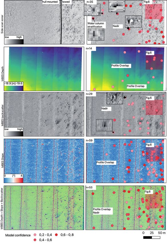
Ocean engineering
Consulting

                                               from space into depth
                                        Realise your projects in cooperation with our hydrographic services

                                                                Our hydrography engineers are happy to develop
                                                                systems tailored exactly to your needs and to
                                                                provide professional advice and support for
                                                                setting up your systems and training your staff.

                                                                MacArtney Germany benefits from being part of
                                                                the MacArtney Group and enjoys unlimited access
                                                                to cutting-edge engineering competences and
               CTDs & SVPs                                      advanced facilities.

                                                Acoustic
                                                sensors

                                                                   Software

                         Position and
                       motion sensors

                                                                   Integration

             Denmark Norway Sweden    United Kingdom France        Italy   Netherlands         Germany
                      USA   Canada   South America    Australia   Singapore        China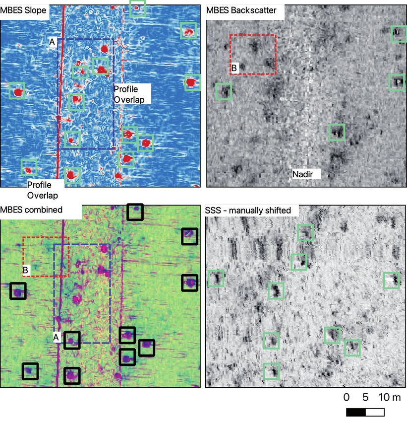
Vorwort
Liebe Leserinnen und Leser,
wir alle nutzen künstliche Intelligenz. Beinahe täg- thischen Arten mittels Deep Learning« (Lütjens
lich. Meist ohne es zu merken. Wenn wir uns von und Sternberg, Seite 18); es geht um den Mangel
Suchmaschinen durchs Web lotsen lassen, wenn an echten Trainingsdaten und um den Versuch,
wir online shoppen. Oder wenn wir für die Suche die künstliche Intelligenz mit synthetischen Bil-
nach dem rechten Weg Navigationssystemen ver- dern zu trainieren (Steiniger et al., Seite 30); und
trauen. es geht um Softwarelösungen, die dank maschi-
In Navigationssystemen steckt künstliche Intel- nellem Lernen neue autonome Anwendungen in
ligenz übrigens gleich dreifach drin. Da wird der der Hydrographie ermöglichen (McPherson Kimø,
kürzeste Weg ermittelt. Da gibt es eine Sprachaus- Seite 36).
gabe. Und da werden aktuelle Verkehrsinformatio- Auffallend ist, dass es bei den KI-Anwendungen
nen mit in die Routenplanung einbezogen. vor allem um das Erkennen von Mustern geht. Und
Ist das nun künstliche Intelligenz? Ja, auch. Aber dass künstliche Intelligenz gar nicht von sich aus
Lars Schiller
eben nicht nur das. Der Begriff lässt sich bislang intelligent ist, sondern erst von Menschen trainiert
nicht wirklich klar definieren. Es geht irgendwie werden muss. Von Science-Fiction keine Spur.
um Informatik, um abgefahrene Technologien Aber umso mehr von Science. Was in diesem Heft
und um immer mehr Anwendungen. präsentiert wird, ist überwiegend Stand der Wis-
Mit Blick auf die Hydrographie schafft hoffent- senschaft, noch nicht Stand der Technik. Die An-
lich diese Ausgabe der Hydrographischen Nach- wendungen finden erst allmählich Einzug in die
richten etwas mehr Klarheit. Wir haben die Frage Praxis.
gestellt, welche Rolle künstliche Intelligenz in der Außerdem im Heft: Die Beiträge von den bei-
Hydrographie spielt. Die Antworten erfahren Sie den für den DHyG Student Excellence Award nomi-
in fünf Fachbeiträgen – zwei davon sind im Peer- nierten Absolventinnen der HCU. Cigdem Askar
Review-Verfahren begutachtet worden – und im vergleicht verschiedene Sedimentecholote für die
Wissenschaftsgespräch mit Professor Alexander Anwendung in flachen Gewässern (Seite 54). So-
Reiterer vom Fraunhofer-Institut für Physikalische phie Andree entwickelt Open-Source-Bibliothe-
Messtechnik IPM in Freiburg (Seite 42). ken für die Prozessierung hydrographischer Daten
In den Fachbeiträgen geht es um Steine auf (Seite 48).
dem Gewässerboden, die künstliche Intelligenz Und Peter Ehlers blickt in einem angemessen
in Messdaten von Fächerecholoten bzw. Seiten- langen Beitrag auf die hundertjährige Geschichte
sichtsonaren erkennen soll (Feldens et al., Seite 6, der IHO zurück (Seite 62).
und Christensen, Seite 24); es geht um die auto- Ich wünsche Ihnen eine erkenntnisreiche Lektü-
matische »Erkennung und Klassifizierung von ben- re dieser Ausgabe.
Hydrographische Nachrichten Chefredakteur:
HN 119 – Juni 2021 Lars Schiller
E-Mail: lars.schiller@dhyg.de
Journal of Applied Hydrography
Redaktion:
Offizielles Organ der Deutschen Hydrographischen Peter Dugge, Dipl.-Ing.
Gesellschaft – DHyG Horst Hecht, Dipl.-Met.
Holger Klindt, Dipl.-Phys.
Herausgeber: Dr. Jens Schneider von Deimling
Deutsche Hydrographische Gesellschaft e. V. Stefan Steinmetz, Dipl.-Ing.
c/o Innomar Technologie GmbH Dr. Patrick Westfeld
Schutower Ringstraße 4
18069 Rostock Hinweise für Autoren und Inserenten:
www.dhyg.de > Hydrographische Nachrichten >
ISSN: 1866-9204 © 2021 Mediadaten und Hinweise
HN 119 — 06/2021 3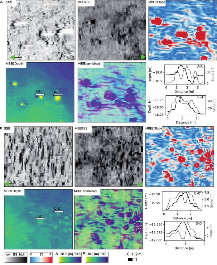
Sonic 2020                         Sonic 2022

       Sonic 2024                         Sonic 2026

     Beispiellose Leistungsfähigkeit mit 256 Beams und 1024
     Soundings bei 160° Öffnungswinkel (einstellbar) und einer Pingrate
     von 60 Hz
     Breitbandtechnologie mit Frequenzwahl in Echtzeit zwischen 200
     bis 400 kHz sowie 700 kHz optional
     Dynamisch fokussierende Beams mit einem max. Öffnungswinkel
     von 0,5° x 1° bei 400 kHz bzw. 0,3° x 0,6° bei 700 kHz
     Höchste Auflösung bei einer Bandbreite von 60 kHz, bzw. 1,25 cm
     Entfernungsauflösung
     Kombinierbar mit externen Sensoren aller gängigen Hersteller
     Flexibler Einsatz als vorausschauendes Sonar und der Fächer ist
     vertikal um bis zu 30° schwenkbar
     Zusätzliche Funktionen wie True Backscatter und Daten der
     Wassersäule
     MultiSpectral Modus™, der es den R2Sonic-Systemen ermöglicht,
     Backscatter Daten mehrerer Frequenzen in einem einzigen Durch-
     lauf zu sammeln

     Nautilus Marine Service GmbH ist der kompetente Partner in
     Deutschland für den Vertrieb von R2Sonic Fächerecholotsystemen.
     Darüber hinaus werden alle relevanten Dienstleistungen wie Instal-
     lation und Wartung kompletter hydrographischer Vermessungssys-
     teme sowie Schulung und Support für R2Sonic Kunden angeboten.
     R2Sonic ist ein amerikanischer Hersteller von modernen Fächerecho-
     loten in Breitbandtechnologie. Seit Gründung des Unternehmens
     im Jahr 2009 wurden weltweit bereits mehr als 1.500 Fächerlote
     ausgeliefert und demonstrieren so eindrucksvoll die
     außergewöhnliche Qualität und enorme Zuverlässigkeit dieser
     Vermessungssysteme.

Nautilus Marine Service GmbH · Alter Postweg 30 · D-21614 Buxtehude · Phone: +49 4161-559 03-0 · info@nautilus-gmbh.com
R2Sonic, LLC · 5307 Industrial Oaks Blvd. · Suite 120 · Austin, Texas 78735 · U.S.A. · Phone: +1-512-891-0000 · r2sales@r2sonic.com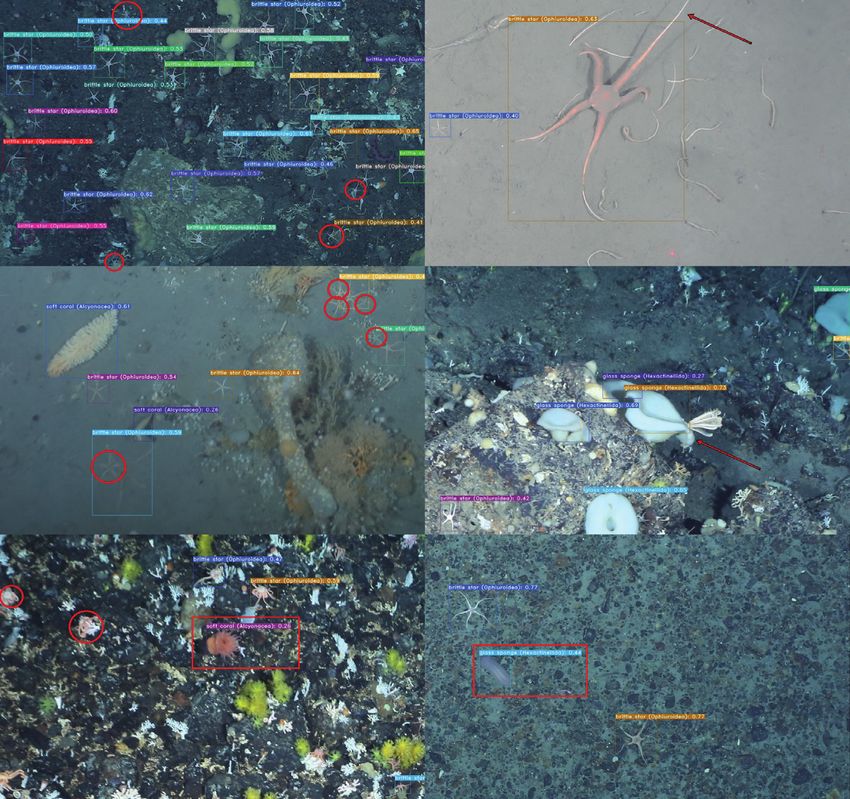
Inhaltsverzeichnis

KI in der Hydrographie
           Bolder detection I
            6 Automatic detection of boulders by neural networks
               A comparison of multibeam echo sounder and side-scan sonar performance
               A peer-reviewed paper by PETER FELDENS, PATRICK WESTFELD, JENNIFER VALERIUS,
               AGATA FELDENS and SVENJA PAPENMEIER

           Image classification
            18 Deep learning-based detection of marine images
               and the effect of data-driven influences
               A peer-reviewed paper by MONA LÜTJENS and HARALD STERNBERG

           Boulder detection II
            24 Automatic boulder identification in side-scan sonar
               An article by JESPER HAAHR CHRISTENSEN

           Synthetische Trainingsdaten
            30 Erzeugung von synthetischen Seitensichtsonar-Bildern mittels Generative Adversarial Networks
               Ein Beitrag von YANNIK STEINIGER, JANNIS STOPPE, DIETER KRAUS und TOBIAS MEISEN

           Autonomous operations
            36 AI is enabling a transformation toward autonomous hydrographic operations
               An article by SARAFINA MCPHERSON KIMØ

           Wissenschaftsgespräch
           42 »Die riesigen Flächen unterhalb der Wasseroberfläche bilden
               das perfekte Szenario für KI-basierte Ansätze«
               Ein Wissenschaftsgespräch mit ALEXANDER REITERER

           DHyG Student Excellence Award I
           48 Interactive processing of MBES bathymetry and backscatter data
              using Jupyter Notebook and Python
              An article by SOPHIE ANDREE

           DHyG Student Excellence Award II
           54 Comparison of different sub-bottom profiling systems to be
              used in very shallow and tide-influenced areas
              A case study in the backbarrier tidal flat of Norderney, Germany
              An article by CIGDEM ASKAR

           Company presentation
            60 Meeting requirements for new types of on-demand survey campaigns
               An article by ANDRES NICOLA and DANIEL ESSER

           IHO anniversary
            62 100 years of international cooperation in hydrography
               An article by PETER EHLERS

           Die nächsten Fokusthemen
             		 HN 120 (Oktober 2021)         Habitatkartierung

             		 HN 121 (Februar 2022)		       Häfen und Verkehre der Zukunft

             		 HN 122 (Juni 2022)		          Meerestechnik

HN 119 — 06/2021                                                                                                   5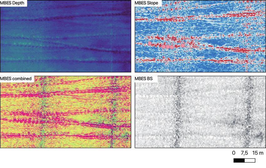
Boulder detection I                                                                                                    DOI: 10.23784/HN119-01

Automatic detection of boulders
by neural networks
A comparison of multibeam echo sounder
and side-scan sonar performance
An article by PETER FELDENS, PATRICK WESTFELD, JENNIFER VALERIUS, AGATA FELDENS and SVENJA PAPENMEIER

Neural networks show great promise in the automatic detection of boulders on the
seafloor. Maps derived from bathymetric data show better performance compared to
backscatter mosaics in this study. However, we find the lack of training data ground-
truthed to a high standard the largest challenge for automated object detection based
on acoustic data.

                                   boulder detection | neural networks | hydrographic surveying | bathymetry | backscatter
                                   Erkennung von Felsbrocken | neuronale Netze | Seevermessung | Bathymetrie | Backscatter

                                   Neuronale Netze sind sehr vielversprechend bei der automatischen Erkennung von Felsbrocken auf dem
                                   Meeresboden. Aus bathymetrischen Daten abgeleitete Karten zeigen in dieser Studie eine bessere Leis-
                                   tung im Vergleich zu Rückstreumosaiken. Die größte Herausforderung für die automatische Objekterken-
                                   nung auf Basis akustischer Daten ist jedoch der Mangel an Trainingsdaten, die auf einem hohen Standard
                                   erprobt sind.

Authors                            1 Introduction                                          ity and generalisation. Against a background of
Dr. Peter Feldens, Agata           Multibeam echo sounders (MBES) have been used           increasing user requirements (e.g. nautical infor-
Feldens and Dr. Svenja             for decades to provide high-quality bathymetric         mation service needs a consistent separation of
Papenmeier work at the             maps of the seafloor (Lurton 2002; Augustin et al.      seabed and boulders for chart production; marine
Leibniz Institute for Baltic Sea   1996; Pickrill and Todd 2003). The German Hydro-        spatial planning requires information about condi-
Research Warnemünde.               graphic Office (Federal Maritime and Hydrograph-        tions on the seabed to assess the impact of off-
Dr. Patrick Westfeld and           ic Agency, BSH) collects bathymetry and detects         shore construction projects) and the compliance
Jennifer Valerius work at          objects underwater by vessel-mounted MBES               with international standards (IHO S-44 Order 1a
the Federal Maritime and           systems (Dehling and Ellmer 2012). The data sur-        and 1b require the reliable detection of obstacles
Hydrographic Agency (BSH) in       veyed in German waters are processed into official      along all main shipping routes), automation of the
Rostock and Hamburg.               nautical charts and nautical publications to ensure     processing chain is indispensable in terms of ac-
                                   navigational safety at sea. Accurate and reliable in-   curacy, reliability and reproducibility of the results.
peter.feldens@io-warnemuende.de    formation of seabed’s topography further forms a        It is also required in the sense of an efficient evalu-
                                   decisive basis for political and technical decisions    ation of large areas.
                                   relating to the sea, including applications depend-         Next to hydrographic applications, recent de-
                                   ing on spatio-temporal-resolved 3-D geodata.            velopments in habitat mapping require the de-
                                   Echo sounding is a measurement technique al-            tection of cobbles and larger hard substrates. The
                                   lowing for the 3-D reconstruction of the surface of     identification of marine hard substrates based on
                                   the seafloor and all objects located on it. As a pri-   acoustic remote sensing is important for the de-
                                   mary result, a digital surface model (DSM) is avail-    tection, delineation and ecological assessment of
                                   able. During the following data processing chain        seafloor habitats (Papenmeier et al. 2020) as well
                                   conducted at BSH, the task is to separate between       as for marine spatial planning. This need is ac-
                                   the surface measured and the actual seabed, to          counted for in several international frameworks,
                                   derive a digital terrain model (DTM) of the seafloor.   such as the Convention on Biological Diversity
                                   The detection and extraction of boulders are chal-      and the Marine Strategy framework directives.
                                   lenging. At BSH, it is realised in a semi-automatic     Boulder detection in the German Baltic and the
                                   process based on geometric filtering, with interac-     North Sea for these purposes is done using side-
                                   tive post-processing and a final visual inspection      scan sonar (SSS) systems. Next to the ease of op-
                                   by well-trained experts. This procedure is time-        eration over large scales, the survey geometry
                                   consuming and error-prone because of subjectiv-         of a side-scan sonar, towed above the seafloor,

6                                                                                                              Hydrographische Nachrichten
Peer-reviewed paper                                                                                                                 Boulder detection I

Fig. 1: Location of the investigation site west of Fehmarn (left). Water depths in the area range between 16 m and 25 m (centre),
dashed lines are the survey lines run during MBES data collection. Right: Slope calculated from the local bathymetry

aids the detection of small objects. Both for man-                2 Methods
ual and automatic methods, boulder detection
was found to be more reliable, with an increas-                   2.1 MBES
ing number of pixels forming an object’s repre-                   Multibeam echo sounder data were collected in
sentation in backscatter (BS) mosaics (Feldens                    summer 2019 from the hydrographic survey ves-
et al. 2019). Acoustic shadows, which form be-                    sel VWFS Deneb, operated by BSH, by a state-of-
hind boulders, increase the number of pixels of                   the-art MBES system Teledyne-Reson Seabat 7125-
boulder representations in backscatter mosaics.                   SV2. The system operates at 400 kHz with a 140°
Shadow sizes increase with grazing angle, thus                    opening angle, a pulse length of 300 µs and 512
favouring towed sonar systems (Papenmeier et                      beams per swath. The seafloor of the study area
al. 2020). Therefore, while the spatial resolution                (Fig. 1, left) was fully covered by 50 survey lines
of modern MBES derived backscatter information                    with 100 % overlap (Fig. 1, centre). The software
can rival that of side-scan sonar systems in many                 Teledyne PDS was used for real-time data acquisi-
relevant practical applications (depending on                     tion. A combined GNSS (Global Navigation Satellite
water depth), their survey geometry is unfavour-                  Systems; good global but poor relative accuracy)
able for boulder detection in backscatter data.                   and INS (Inertial Navigation System; good local ac-
However, the pixel-perfect co-registration of                     curacy but drifts without external reference) forms
depth and backscatter and derived data sets may                   the basis for an accurate and reliable real-time di-
offset this disadvantage and facilitate boulder                   rect georeferencing of MBES measurements. MBES
detection based on MBES data. Considering the                     instruments require an accurate portrayal of the
interpretation of extensive areas, human experts                  sound speed structure of the water column. In this
have difficulties in combining information of mul-                campaign, the distribution of water sound velocity
ti-dimensional data sets, while machine learning                  was determined by continuous profile measure-
algorithms are less limited by dimensionality and                 ments using the multi-parameter online probe
more efficient (Yokoya et al. 2017).                              Sea & Sun Technology CTD 60Mc. Bathymetry data
   In the last decade, object detection frame-                    were processed using Teledyne CARIS HIPS & SIPS.
works based on convolutional neural networks                      The processing chain holds techniques for i.a. cor-
(CNN) were applied to different topics, including                 rection of sound velocity induced effects, calcula-
remote sensing in the earth sciences (Ghamisi et                  tion of a georeferenced 3-D point cloud, genera-
al. 2017; Zhu et al. 2017) with great success. CNNs               tion of 3-D surface representation of the bottom
were used to find boulders in side-scan sonar                     topography, outlier detection and filtering.
backscatter mosaics, showing performance com-                        To create backscatter grids with a resolution of
parable to human experts in areas of moderate to                  0.25 m based on the multibeam echo sounder
good data quality (Feldens et al. 2019). It is the aim            data provided as s7k-files, angular variations in
of this case study to compare the performance of                  intensities were removed using the open-source
multibeam echo-sounder and side-scan sonar to                     processing toolbox MB-System (Caress and
image boulders in single-band and multi-band                      Chayes 1996). A grazing angle of 40° (here, minor
data sets including depth, slope and backscatter                  variations in incidence angle have little effect on
intensity. An object detection framework based                    backscatter intensity) was used as a reference
on a neural network is used to identify boulders                  angle. A low pass Gaussian mean filter stretching
in the data sets, and the results are compared with               five samples in the across-track and three samples
the interpretation of human experts.                              in the along-track direction was applied once to

HN 119 — 06/2021                                                                                                                                     7
Boulder detection I
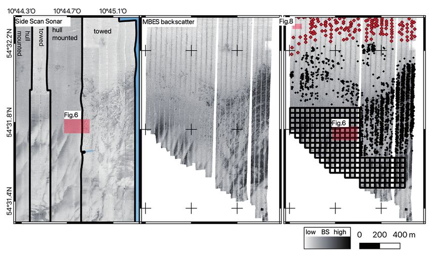
Fig. 2: Left: Side-scan sonar backscatter mosaic (0.25 cm pixel size) used for boulder
classification in this study. Centre: Multibeam echo sounder backscatter mosaic.
Right: Location of the boulders (black dots) and empty image examples (red dots) used for training of the models
based on multibeam echo sounder data. The red box represents the test area for the manual identification of
individual boulders in Fig. 6 and false positives examples in Fig. 8, respectively. The raster grid used for the manual
determination of boulders densities is indicated
the data to remove high frequency speckle noise. 4.5 kn. Using a swath-width of 200 m the profile
Data gaps of up to 1.25 m were interpolated. The distance was set to 180 m to allow an overlap of
grid was built by applying a Gaussian Weighted approximately 10 % at the edges.
Mean. As available profiles are overlapping, sam- Processing of the backscatter amplitudes was
ples of higher grazing angles were given an in- done with the software package SonarWiz 7.3.
creased priority during gridding. Profiles were run Only the higher frequency of the CSS-2000 has
in both N-S and S-N directions on the same pro- been used (600 kHz). The 4300 MPX used a fre-
file track. For the backscatter maps, one of these quency of 410 kHz. After bottom tracking and em-
directions was used, the other line was discarded. pirical gain normalisation, the data of the towed
Backscatter intensities were clipped at the 0.2 % system additionally required a correction of the
and 99.8 % percentile to improve image contrast. navigation data. The sheave offset was adjusted,
In this study, higher backscatter intensities are dis- and a layback correction was executed basing on
played in darker colours. All backscatter intensities data of a cable counter and a pressure sensor. To
are uncalibrated, relative values (Lamarche and generate a final backscatter mosaic both data sets
Lurton 2018) and were exported as 8-bit greyscale were merged. The overlapping profiles were cut at
mosaics following processing. Multi-band images the edges as far as possible without causing gaps.
of MBES-derived grids of backscatter, slope and Finally, a mosaic (8-bit greyscale) with a spatial res-
depth were created using the open source GDAL olution of 25 cm was exported (Fig. 2, left).
utilities (GDAL/OGR contributors 2021), by plac-
ing slope information in the green image channel 2.3 Manual boulder count
(Fig. 1, right), backscatter information in the red im- Two experienced human interpreters did a manual
age channel (Fig. 2, centre) and depth values in the count of individual boulders in a test area (Fig. 2,
blue image channel (Fig. 1, centre). red box) based on the side-scan sonar mosaics.
Human interpreters generally recognise boulders
2.2 SSS by an increased backscatter intensity facing to-
The side-scan sonar data were recorded in May wards the side-scan sonar, followed by an acoustic
2019 during cruise #164 with the vessel VWFS shadow forming behind. The human interpret-
Deneb. The Edgetech CSS-2000 was towed at an ers were not involved in picking the training data
altitude of approximately 12 ± 3 m above the sea- for the neural networks. To interpret larger areas,
bed. Due to technical problems with the CSS-2000 a raster approach is used. For 50 m × 50 m cells
a change to the hull-mounted side-scan sonar (Fig. 2, black raster grid), the same human experts
(Edgetech 4300 MPX) became necessary dur- decided whether it includes no boulders, one to
ing the cruise (Fig. 2 shows the coverage of both five boulders, or over five boulders. This procedure
data sets). The vessel speed varied between 4 and is in line with currently published recommenda-
8 Hydrographische Nachrichten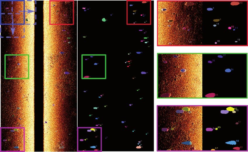
Boulder detection I

tions for mapping geogenic reefs (Heinicke et al.,        backbone and neck) to extract object features and
in press), used to characterise geogenic reefs over       divide the input image into grids at three different
larger areas. The agreement between the human             resolutions. For each grid cell at each resolution,
experts is calculated using the F₁ score of the re-       it predicts the probability that the cell includes a
sulting confusion matrix. An F₁ score of 1.0 indi-        learned object within anchor boxes of predefined
cates perfect agreement, while the lowest value is        size. These probabilities and the corresponding
0, when either precision or recall are 0. The F₁ score    bounding box coordinates are the output of the
is calculated from the confusion matrix by F₁ = 2 ×       trained model. YOLO networks are available in dif-
(precision × recall) / (precision + recall). Values for   ferent configurations of the backbone, of which
each class (no boulders, one to five boulders and         we here utilise the standard configuration of YOLO
more than five boulders) were averaged.                   version 4.

2.4 Automatic boulder count                               2.4.2 Model training and application
2.4.1 Neural network                                      To create the training data sets, a human inter-
Artifical neural networks are composed of series          preter identified bounding boxes of boulders in
of interconnected layers of artificial neurons. In        training areas in QGIS 3.16. Boulders were required
a trained neural network, input signals are trans-        to have a shadow. The boulders were exported as
formed by changing weights at each connection,            an SQLite database. The training database for the
until the last layer of the network reports the re-       SSS model includes 13,847 boulder instances. A
sult of the computation. Convolutional neural             model was trained on a data set with an empha-
networks are a subset of neural networks and              sis on small boulders comprising only a few pixels.
were developed for image classification with over-        This data set comprises 4,070 entries. The MBES
whelming success. While the architecture of CNNs          training database was only started with the inves-
varies, all include a series of convolutional layers,     tigation site reported here (Fig. 2). It is not possible
that operate by convolving a small part, often 3 × 3      to use the same training data sets for MBES and
pixels, of the underlying image (or the output of an      SSS models, since the position accuracy of the
earlier layer in the network) with weights initialised    side-scan sonar is not good enough to co-locate
at random. This assumes that pixels in close vicin-       features of only a few pixels in size. Therefore, the
ity are more likely to form patterns significant for      MBES training data set comprises 2,654 instances
the image context than those pixels with greater          of boulders (Fig. 2), with typical sizes of 3 × 3 to
distance. The weights are adjusted during model           8 × 15 pixels including shadows. The training mo-
training with annotated images to minimise a loss         saics were cut into small georeferenced images of
function. Loss functions compare the predictions          64 × 64 pixels (corresponding to approximately
of the neural network to the annotations. To allow        16 m × 16 m in this study), overlapping by six pix-
CNNs learning non-linear features, activation func-       els to minimise the number of training boulders
tions change the output of layers in the network,         that are cut by image boundaries. In the following,
while regular downsampling of the image size al-          the pixel coordinates of the annotated examples
lows the network to learn features of larger scales.      were calculated and used as an input for training.
   The automated boulder count was done using             Besides the annotated boulder examples, 182 ex-
the YOLO (You Look Only Once) framework, de-              amples of empty images (defined as containing no
veloped by Joseph Redmon (Redmon et al. 2015),            boulders) were selected for the MBES data set and
with the current implementation available under a         2,349 examples of empty images for the SSS data
permissive license on GitHub (https://github.com/         set.
AlexeyAB/darknet). Lary et al. (2016) and Schmid-            For training, we used the YOLO network ver-
huber (2015) give a detailed description of convo-        sion 4, in contrast to earlier case studies that used
lutional neural networks and their application for        the two-stage RetinaNet framework (Lin et al.
image interpretation.                                     2017). We adhered to suggestions published on
   The YOLO network was developed for object              the project’s GitHub page and changed the de-
detection. To identify and locate different objects       fault configuration of the YOLO network. There-
in images is more complicated than the classifica-        fore, the maximum number of training batches
tion of entire images and requires a different net-       was reduced to 6,000 for MBES models and 24,000
work architecture. YOLO is a one-stage detector,          for SSS models, the number of classes reduced to
meaning it analyses images in one pass (hence the         one, and the filter number of the convolutional
abbreviation, You Only Look Once) while keeping           layers before the object detection layers reduced
high accuracy. One-stage detectors are a faster           to 18. Images were magnified to 512 × 512 pixels
approach compared to other object detection               before training. Random variations in hue, expo-
frameworks that rely on multiple stages for object        sure and saturation applied to the image were re-
detection in images. The YOLO architecture is de-         duced from their standard settings to 0.1. The size
scribed by Bochkovskiy et al. (2020). In principle, it    of the input image was changed by 40 % every
uses a series of different convolutional layers (the      ten batches at random, and the size and aspect

HN 119 — 06/2021                                                                                                                      9
Boulder detection I

 Fig. 3: The appearance of boulders in the different data sets. A) At a distance of 45 m to the nadir individual boulders are recognised in SSS backscatter.
 The same boulders (27 m to the nadir) are more difficult to recognise in MBES backscatter. The boulders are visible in bathymetry, slope, and combined
 data sets. B) Small boulders as imaged in the outer part (75 m to nadir) of a side-scan sonar swath. The characteristic boulder pattern is hard to recognise
 and appears smeared in the along-track direction, due to yaw movements or decreasing along-track resolution. The appearance of boulders is difficult to
 interpret in MBES (20 m to nadir) backscatter, but the objects are recognised in slope, bathymetry and combined data sets. The position of SSS images was
 shifted by several metres to account for positional differences to the MBES. The green arrow points to the nadir. SSS data was recorded with a CSS-2000

10                                                                                                                           Hydrographische Nachrichten
Boulder detection I

ratio were also changed by ±60 % for each image.                 up also controls the local slope shown in Fig. 1.
The optimal anchor sizes for the YOLO network                    While high pixel-to-pixel slopes exceeding 60° at
were calculated. 15 % of the training samples were               maximum prevail in the areas of glacial lag depos-
randomly selected for validation and used to cal-                its due to the presence of boulders and near the
culate the average precision for the boulder class               trawl marks, the remaining area is flat with slope
(AP) of the different networks. After the image set              values below 2°.
for validation was separated, a Python script ro-                   Based on a visual inspection, we find most boul-
tated every image in 45° steps to account for vari-              ders in the area composed of glacial lag deposits,
able survey directions. The training took place on               with some also present in the sandy facies. The
a NVIDIA 2080 TI graphic card (11 GB RAM). Training              boulders have different characteristics in the data
of the MBES models required about twelve hours                   sets that are displayed in Fig. 3. In the SSS-derived
for the MBES models and 40 hours for the large                   backscatter mosaics, boulders can be recognised
SSS model.                                                       by a high backscatter front, an intermediate in-
  For model application, the training procedure is               tensity signal behind and an acoustic shadow at
reversed. The (single or multi-band) mosaic is cut               the back, relative to the side-scan sonar position.
into small georeferenced image tiles of 64 × 64                  However, small boulders are often more difficult to
pixels. Threshold values for include objects were                interpret. This is caused either by their small size
set to 0.2 for all models except the SSS model for               or their position in the outer part of the swath (a
small objects, which was set to 0.35. The model is               combination of which is shown in Fig. 3B). In addi-
run on these small tiles. The detection of objects               tion, artefacts in side-scan sonar data can resem-
on a single image requires about 10 ms on an                     ble smaller boulders. Such artefacts include scatter
NVIDIA 2080 TI. The pixel-coordinates of the result-             from water column stratification or areas near the
ing bounding boxes are converted to geographic                   side-scan sonar nadir.
coordinates and displayed using QGIS. To emulate                    In MBES-derived backscatter, boulders are rec-
the raster approach used by human experts to                     ognised by an increase in backscatter intensity
cover large areas, detected boulders in each grid                compared to the surrounding seafloor (Fig. 3) but
cell are counted.                                                are often lacking a pronounced acoustic shadow.
                                                                 The backscatter representation of boulders is less
3 Results                                                        distinct compared to SSS imagery in close to inter-
                                                                 mediate distance to the nadir. Boulders are imaged
3.1 Local geology and appearance of boulders                     as circular to elliptic features in maps of the local
Water depths in the investigation site (approxi-                 slope. Slope values for boulders range from 3.5° to
mately 2 km²) vary between 16 m and 25 m, with                   more than 60° degrees, related to the large vari-
depths increasing towards the north. Backscatter                 ety of boulder shapes in transported lag deposits
maps derived from MBES and SSS show different                    transported by glaciers. Also, boulders may be par-
seafloor facies at the site (Fig. 2), with fine-grained          tially buried in the subsurface. However, not all cir-
deposits and intensive disturbance by bottom                     cular features correspond to increased backscatter
trawling activities in the north (low backscatter).              intensities, for example in the areas of overlapping
High backscatter intensities characterise glacial                profiles. In MBES-derived maps of depth, boulders
lag deposits towards the south and east. A high                  are displayed as circular features elevated 2.5 cm
number of boulders are part of these deposits. In-               to over 50 cm compared to the adjacent seafloor.
termediate backscatter intensities towards south
and west characterise fine to medium sands and                   3.2 Manual boulder identification
partial outcrops of glacial lag deposits. In the side-           For a test area of about 30,000 m², two experi-
scan sonar mosaics, which cover a larger area, a                 enced human interpreters picked boulders on the
series of elongated, elevated ridges exist in the                side-scan sonar backscatter mosaic (Fig. 4). The
southeast. The general sedimentological build-                   test area showcases instances of water column

Fig. 4: Manual interpretation of boulder occurrence in the test area based on SSS backscatter data.
The number of identified objects is 26 and 54. Refer to Fig. 2 for location

HN 119 — 06/2021                                                                                                                          11
Boulder detection I
Fig. 5: Top: Number of boulders identified with the raster approach by the slope-model and to human experts.
Bottom: Individual detection of the slope-model are plotted on top of the expert II interpretation. Coloured cell boundaries
visualise the difference in interpretation between the human experts. A) Example of a potential boulder not noticed by
the experts. B) A potential false positive detection of the model. C) Detections near the side-scan sonar nadir, where no
judgment of the model detections is possible. For C, the slope map is shown in addition
stratification on the eastern side, a nadir stripe in F₁ score, measuring the agreement between the
the centre of the area and an overlap of two differ- two experts, is 0.61 based on 196 raster cells.
ent profiles recorded with different side-scan so-
nars towards the west. The experts found 26 and 3.3 Automated boulder detection
54 boulders. No human misinterpreted the water The Average Precision (AP) of the models on the
column artefacts, nadir stripes or overlapping pro- validation data is shown in Table 1. The highest
files as boulders. A higher variability exists in the performance is 64 % by the slope-only model, fol-
outer parts of the swath near the overlapping pro- lowed by a model working on a 3-band data set
files, where the appearance of potential boulders comprising MBES backscatter, slope and depth
varies. The same human experts interpreted boul- with 61 % AP. The MBES backscatter-only model
der densities over a larger area using the raster ap- achieves an AP of 18 %. The side-scan sonar per-
proach applied to 50 m × 50 m cells (Fig. 5). Dense formance is 37 % to 43 %, with the lower AP for the
boulder assemblages were confirmed in the east training data set with a focus on small objects. The
towards the outcropping glacial till, while boulders detections of the best-performing slope-model
are sparse towards west. Corresponding to the dif- are plotted on top of boulder densities as deter-
ferent number of individual boulders found in the mined by human experts (Fig. 5).
test area, expert I identified a larger area covered The resulting detections of the models in the
by one to five boulders compared to expert II. The test area are shown in Fig. 6. The SSS models
find a total of 35 boulders, all including a discern-
Data set Model AP ible shadow on visual inspection. One likely false
MBES SLOPE 64 % positive occurs around water column stratifica-
tion artefacts and one false positive in the nadir
MBES DEPTH SLOPE BACKSCATTER 61 %
region. The MBES backscatter model finds a total
SSS BACKSCATTER large objects 43 % of 29 boulders. Of these, seven have no discern-
ible shadow, while the remaining display at least
SSS BACKSCATTER small objects 37 %
one pixel of acoustic shadows behind. The mod-
MBES DEPTH 36 % el working on the area-wide bathymetric grids
MBES BACKSCATTER 18 % detects 14 boulders with elevations of 6 cm to
40 cm compared to the surrounding seafloor,
Table 1: Overview of performance on the validation data set albeit most boulders smaller than 15 cm are not
(measured in AP) for the different models and data sets recognised in the data set. The slope model finds
12 Hydrographische NachrichtenBoulder detection I 59 objects at the test site, characterised by slopes slope data set. However, several potential boulders ranging from 35° to less than 3.5°. However, most found in the slope data set were not found by the identified boulders show slope values of over 4°. combined model and vice versa, with examples The model running on the combined data set of shown in Fig. 7. Here, a comparison with the in- backscatter, slope and depth detects 53 boulders. dependently recorded side-scan sonar data – bar- Most of these boulders are also recognised in the ring some uncertainty because of the positional Fig. 6: Boulders found by the models in the test area in the different data sets. For the SSS backscatter mosaic, magnified insets show the similarity of small boulders and artefacts due to water column stratification and near- vertical incidence. Refer to Fig. 2 for location HN 119 — 06/2021 13
Boulder detection I

                      inaccuracy that required shifting the side-scan                   4 Discussion
                      sonar mosaic location by a few metres – seems                     The high difference of boulder detection by very
                      to show that the slope data is correct, and these                 experienced human interpreters (Fig. 3) shows
                      objects should have been identified as boulders.                  the need for an objective, automatic method for
                      In contrast, in the northern test area (Fig. 8), circu-           boulder detection. The different count of individ-
                      lar elevated features are identified as boulders by               ual boulders transfers to an agreement of 0.61 (F₁
                      the slope-model. We find similar examples, not                    score) over 196 cells that were interpreted with the
                      displayed here, in areas with remaining outliers in               raster approach. This poses a significant challenge
                      morphological data which have a similar appear-                   both for quantification of model performance
                      ance. Such outliers cause artificial slopes but do                and for the establishment of correctly annotated
                      not affect backscatter data information.                          training images, a problem faced by many other
                         The results of the raster approach using the                   applications of neural networks to remote sensing
                      model with the highest AP (the slope-model) are                   data (Zhu et al. 2017). The same person interpret-
                      shown in Fig. 5. The slope-model identifies be-                   ing the training database and the reference sites
                      tween 0 and 42 boulders in the 50 × 50 m cells.                   for boulder detection (Feldens et al. 2019) partially
                      The agreement with the human experts I and II as                  mitigates the problem. However, this approach
                      measured by the F₁ score for 182 cells (cells where               does not scale to more than one involved person
                      both SSS and MBES data are available) is 0.75 and                 or to applications where objective results without
                      0.63, respectively.                                               interpreter bias are required. Almost no study in-
                                                                                        cludes an extensive ground truthing for boulders

                      Fig. 7: Boulders detected by the MBES-models are displayed. Boulders are verified in the side-scan
                      sonar image, whose position was shifted to account for positional inaccuracies. Near the nadir, potential
                      boulders are not imaged in MBES backscatter data, while present in the slope map (blue rectangle).
                      Vice versa, the backscatter map displays increased backscatter intensities in areas where no increased
                      slope exists (red rectangle). No boulders are detected in both areas by the combined model working on
                      depth-slope and backscatter channels. Refer to Fig. 6 for colour scales

14                                                                                                             Hydrographische Nachrichten
Boulder detection I Fig. 8: Test area composed of fine sediments with a marked impact of bottom trawling activity. Because of the fine sediment composition, it can be assumed no boulders are present in this area. The model working on slope data detects several false positives in the area, while models running on backscatter, depth and the combined multi-band image report no false positives. Refer to the northwest of Fig. 2 for location in acoustic data, and – except for obvious instanc- model to detect small boulders – as required by es – the interpretation of a human interpreter of regulations – is increased, the amount of false what is and what is not a boulder varies based on positive identifications increases as well. Because his/her experience, with no possibility to judge of the absence of well ground-truthed reference what is the correct interpretation. The appearance sites, a calculation of meaningful precision-recall and visibility of boulders in backscatter data can curves to find optimal threshold values is not pos- change with swath width and incidence angle (Pa- sible. Tuning the threshold level of the model to penmeier et al. 2020; von Rönn et al. 2019). While a the local conditions (e.g., the number of artefacts methodological description on how to assess geo- in the data) is done manually, which is a subjec- genic reefs exists (Heinicke et al., in press), it de- tive procedure. A possible solution is to include fines no sufficient criteria to decide which objects nadir and water column stratification effects as are to be identified as boulders in acoustic data. distinct classes and define these areas as insuffi- Still, our case study allows qualitative insight cient for boulder detection. While MBES snippet- into the advantages and disadvantages of SSS derived backscatter data is not affected by water and MBES-based boulder mapping by neural net- column stratification and is used for object detec- works. To mitigate the impact on AP for the dif- tion (e.g., Kunde et al. 2018), individual boulders ferent models, a single person confirmed all sam- are not displayed in the specular regime (Fig. 7) at ples in the training database used for this study. near-vertical incidence angle and are resolved in Therefore, model performance is only compared less detail compared to side-scan sonar images in relative to the interpretation of the acoustic data the data (Fig. 2). The loss of detail may be caused by one human expert and not to the true seafloor by a different along-track resolution due to dif- conditions. Both SSS and MBES systems supply ferent opening angles of the used systems (0.5° backscatter information. A problem of SSS-based at 400 kHz for the Reson 7125, CSS-2000: 0.26° boulder detection are artefacts (Wilken et al. 2012), at 600 kHz, respectively 0.29° at 410 kHz for the e.g., near the nadir or in areas of water column 4300 MPX). Combined with the less pronounced stratification that can in their structure resemble acoustic shadows, the AP of the MBES backscatter small boulders (Fig. 6). Due to the requirements to model data set, therefore, is worse compared to detect tiny objects comprising only 7 to 9 pixels in the model trained on side-scan sonar backscatter the examples shown here and even less if objects data (Table 1). MBES-based backscatter maps can- of 25 cm in size are to be detected in acoustic data not be recommended as the principal data source (von Rönn et al. 2019), there is limited information for boulder detection based on our case study. to differentiate between artefacts and real objects. An obvious problem related to the use of MBES This causes a trade-off during the training of side- bathymetry and derived slope values is the re- scan sonar-based models: if the sensitivity of the quired thorough cleaning of the data, with outli- HN 119 — 06/2021 15
Boulder detection I

                      ers or morphological features having similarities          possible (Beisiegel et al. 2019), and changing depth
                      to small boulders in slope maps. An example of             intervals between different sites (and thus chang-
                      such morphological feature in the German Baltic            ing resolution in colour-coded depth images) may
                      Sea is related to bottom trawling (Fig. 8). The trawl      be problematic. We suggest exploring the use of
                      doors create steep local, almost circular morpho-          further depth-derived information, such as the
                      logical features when lifted off the seafloor. These       bathymetric position index, or texture parameters
                      features are misinterpreted by the slope-only              derived from backscatter mosaics in the future.
                      model as boulders. The backscatter model cor-                 Models working on a combination of depth,
                      rectly ignores these features. The combination of          slope and backscatter data produced false nega-
                      backscatter and slope data also prohibit false posi-       tives in the near-nadir region, as boulders are not
                      tives in the combined model. Therefore, while the          imaged in the backscatter channel. They also show
                      AP of the slope model is the best on the valida-           fewer false positives and are less susceptible to re-
                      tion data overall (Table 1), it also produced unde-        maining outliers in bathymetric data. Therefore,
                      sirable false positives in areas where boulders are        while the performance of the joint depth-slope-
                      very unlikely to appear (Fig. 7). The pixel-perfect        backscatter data set is worse than for the slope-
                      coregistration of depth and backscatter informa-           only model (due to validation examples in the
                      tion by multibeam echo sounders can mitigate               nadir region) in our case study, its inherent robust-
                      this downside. Being the best model in our case            ness to false positives by combining independent
                      study, the slope-model results were compared               data sets makes it the method of choice for practi-
                      with the human raster-based interpretation of a            cal applications in the future. Ideally, and needed
                      larger area. The F₁ score of the model compared to         for many commercial applications anyway, an over
                      the human experts is 0.75 and 0.62. Both scores are        100 % overlap would remove the near-vertical in-
                      higher than the score for the direct comparison of         cidence backscatter data and is expected to im-
                      the human experts, although the number of raster           prove model results. Multi-band images with cali-
                      cells counted is not identical due to the different        brated backscatter data collection (Lamarche and
                      extension of available SSS and MBES data. Position-        Lurton 2018) would also allow for a quantitative
                      al inaccuracies between the side-scan sonar and            definition of boulders, e.g., by measuring increase
                      multibeam echo sounder data of approximately               of backscatter intensity in addition to local slope
                      5 m may negatively impact the comparison of cells          and local bathymetric position index.
                      where boulders are situated close to the edges. In
                      hindsight interpretation of the model-human dif-           5 Conclusion
                      ferences, potential errors on both sides were iden-        Our case study shows that boulders are detected
                      tified (examples shown in Fig. 5). In addition, the        with higher precision in bathymetric data com-
                      slope data is less affected than backscatter inten-        pared to backscatter mosaics recorded by either
                      sity by survey geometry and finds boulders that            multibeam echo sounder or side-scan sonar. The
                      could not be identified in the side-scan sonar data        results of the best model are comparable to the
                      because they are located close to the nadir.               range of results achieved by human interpret-
                         The poorer performance of the MBES depth-de-            ers. We recommend combining bathymetry and
                      rived model compared to the slope model is not             backscatter data into a multi-band image to limit
                      surprising, given that the maximum resolution of           false positive detections. However, the limiting
                      the input image is the regional depth interval di-         factor for the automated detection of boulders in
                      vided by the available discrete pixel values. In our       acoustic data is not the technology, but the do-
                      study, this is 9 m divided by 256 (28 bpp, bit per         main knowledge and the availability of accurately
                      pixel), artificially limiting the vertical resolution to   annotated training images. Future activities should
                      ca. 0.035 m in the single band 8-bit image. Given          involve the careful choice of sites for ground-truth-
                      that many boulders have smaller elevations (Fig. 2)        ing and acoustic surveys, to create a high-quality
                      and are visible in slope maps, the performance             training data set. //
                      of the depth model is good and may have great
                      potential for models operating on point clouds             Acknowledgment
                      and derived statistics which became available in           The authors thank Elham Al-Akrami for initial prep-
                      the last years (Held and Schneider von Deimling            aration of MBES-related training data set, and Mer-
                      2019; Guo et al. 2020). The advantages and disad-          le Hennig for support in digitising boulders on the
                      vantages of including absolute depths as an input          SSS mosaics. We thank the crew of VWFS Deneb
                      channel for neural networks must be considered,            for their great support during the measurement
                      however. In the Baltic Sea, for example, finding           campaigns, and the two reviewers who provided
                      boulders in deeper muddy basins is unlikely, but           helpful and constructive comments.

16                                                                                                  Hydrographische Nachrichten
Boulder detection I References Augustin, Jean-Marie; Raymond Le Suavé et al. (1996): Lamarche, Geoffray; Xavier Lurton (2018): Recommendations Contribution of the multibeam acoustic imagery to for improved and coherent acquisition and processing of the exploration of the sea-bottom. Marine Geophysical backscatter data from seafloor-mapping sonars. Marine Researches, DOI: 10.1007/BF00286090 Geophysical Research, DOI: 10.1007/s11001-017-9315-6 Beisiegel, Kolja; Franz Tauber et al. (2019): The potential Lary, David J.; Amir H. Alavi et al. (2016): Machine learning in exceptional role of a small Baltic boulder reef as a solitary geosciences and remote sensing. Geoscience Frontiers, habitat in a sea of mud. Aquatic Conservation: Marine and DOI: 10.1016/j.gsf.2015.07.003 Freshwater Ecosystems, DOI: 10.1002/aqc.2994 Lin, Tsung-Yi; Priya Goyal et al. (2017): Focal Loss for Dense Bochkovskiy, Alexey; Chien-Yao Wang, Hong-Yuan Mark Liao Object Detection. arxiv: 1708.02002 (2020): YOLOv4: Optimal Speed and Accuracy of Object Lurton, Xavier (2002): An introduction to underwater Detection. arXiv: 2004.10934 acoustics: principles and applications. Springer Science & Caress, David W.; Dale N. Chayes (1996): Improved processing Business Media of Hydrosweep DS multibeam data on the R/V Maurice Papenmeier, Svenja; Alexander Darr et al. (2020): Ewing. Marine Geophysical Researches, DOI: 10.1007/ Hydroacoustic Mapping of Geogenic Hard Substrates: BF00313878 Challenges and Review of German Approaches. Dehling, Thomas; Wilfried Ellmer (2012): Zwanzig Jahre Geosciences, DOI: 10.3390/geosciences10030100 Seevermessung seit der Wiedervereinigung. AVN Vol. 119, Pickrill, Richard A.; Brian J. Todd (2003): The multiple roles Nr. 7, S. 243–248 of acoustic mapping in integrated ocean management, Feldens, Peter, Alexander Darr et al. (2019): Detection of Canadian Atlantic continental margin. Ocean & Coastal Boulders in Side Scan Sonar Mosaics by a Neural Network. Management, DOI: 10.1016/S0964-5691(03)00037-1 Geosciences, DOI: 10.3390/geosciences9040159 Redmon, Joseph; Santosh Divvala et al. (2015): You Only Look GDAL OGR contributors (2021): GDAL/OGR Geospatial Data Once: Unified, Real-Time Object Detection. DOI: 10.1109/ Abstraction software Library. Open Source Geospatial CVPR.2016.91 Foundation Schmidhuber, Juergen (2015): Deep learning in neural Ghamisi, Pedram; Javier Plaza et al. (2017): Advanced Spectral networks: An overview. Neural Networks, DOI: 10.1016/j. Classifiers for Hyperspectral Images: A review. IEEE neunet.2014.09.003 Geoscience and Remote Sensing Magazine, DOI: 10.1109/ von Rönn, Gitta Ann; Klaus Schwarzer et al. (2019): Limitations MGRS.2016.2616418 of Boulder Detection in Shallow Water Habitats Using Guo, Yulan; Hanyun Wang et al. (2020): Deep learning High-Resolution Sidescan Sonar Images. Geosciences; for 3d point clouds: A survey. IEEE Transactions on DOI: 10.3390/geosciences9090390 Pattern Analysis and Machine Intelligence, DOI: 10.1109/ Wilken, Dennis; Peter Feldens et al. (2012): Application of 2D TPAMI.2020.3005434 Fourier filtering for elimination of stripe noise in side-scan Heinicke, Kathrin; Tim Bildstein; Dieter Boedecker (in press): sonar mosaics. Geo-Marine Letters, DOI: 10.1007/s00367- Leitfaden zur großflächigen Abgrenzung und Kartierung 012-0293-z des LRT 1170 »Riffe« in der deutschen Ostsee (Untertyp: Yokoya, Naoto; Claas Grohnfeldt; Jocelyn Chanussot geogene Riffe) (2017): Hyperspectral and Multispectral Data Fusion: Held, Philipp; Jens Schneider von Deimling (2019): New A comparative review of the recent literature. IEEE Feature Classes for Acoustic Habitat Mapping – A Geoscience and Remote Sensing Magazine, DOI: 10.1109/ Multibeam Echosounder Point Cloud Analysis for Mapping MGRS.2016.2637824 Submerged Aquatic Vegetation (SAV). Geosciences, Zhu, Xiao Xiang; Devis Tuia et al. (2017): Deep learning in DOI: 10.3390/geosciences9050235 remote sensing: A comprehensive review and list of Kunde, Tina; Philipp Held et al. (2018): Ammunition detection resources. IEEE Geoscience and Remote Sensing Magazine, using high frequency multibeam snippet backscatter DOI: 10.1109/MGRS.2017.2762307 information. Marine Pollution Bulletin, DOI: 10.1016/j. marpolbul.2018.05.063 HN 119 — 06/2021 17
Image classification DOI: 10.23784/HN119-02
Deep learning-based detection of
marine images and the effect of
data-driven influences
An article by MONA LÜTJENS and HARALD STERNBERG
Throughout recent years convolutional neural networks have been applied for various
image detection tasks. Training data thereby plays an important role for the perfor-
mance of those models. Not only the amount of images is crucial but also the number
of annotations, classes as well as image dimensions. In view of changing underwater
environments, the study of benthic communities is increasingly important especially
in the Southern Ocean as they provide a key link for ecosystem shifts. This study con-
centrates on the automatic detection and classification of benthic species using deep
learning. It could be shown that glass sponges, brittle stars and soft corals could suc-
cessfully be detected even on few input data and highly biased class distributions in
varying underwater scenes. Further analyses considering data-driven influences show
significant performance declines regarding the training on single objects and classes
per image and the evaluation on large image dimensions.
deep learning | automatic detection | underwater imagery | benthos
Deep Learning | automatische Detektion | Unterwasserbilder | Benthos
In den letzten Jahren wurden gefaltete neuronale Netze für verschiedene Aufgaben der Bilderkennung
eingesetzt. Die Trainingsdaten spielen dabei eine wichtige Rolle für die Leistungsfähigkeit dieser Modelle.
Dabei ist nicht nur die Menge der Bilder entscheidend, sondern auch die Anzahl der Annotationen, Klas-
sen sowie die Bilddimensionen. Angesichts sich verändernder Unterwasserumgebungen wird die Unter-
suchung benthischer Lebensgemeinschaften vor allem im Südlichen Ozean immer wichtiger, da sie hier
vor allem sensibel auf Veränderungen reagieren. Diese Arbeit konzentriert sich auf die automatische Er-
kennung und Klassifizierung von benthischen Arten mittels Deep Learning. Es konnte gezeigt werden,
dass Glasschwämme, Schlangensterne und Weichkorallen selbst bei wenigen Eingabedaten und stark
unterrepräsentierten Klassen in unterschiedlichsten Unterwasserlandschaften erfolgreich erkannt werden.
Weitere Analysen zu datengetriebenen Einflüssen zeigen deutliche Leistungseinbußen bei einzelnen Ob-
jekten und Klassen pro Bild während des Trainings und großen Bilddimensionen während der Evaluation.
Authors 1 Introduction an increasing amount of underwater imagery has
Mona Lütjens is Research Global ocean temperature rise and ocean acidifica- emerged raising the need for automatic analytical
Associate at HafenCity tion are ubiquitous and threaten especially benthic methods. Recent research in full automatic detec-
University in Hamburg. communities in the Southern Ocean where many tion and classification of marine images deploy
Harald Sternberg is Professor species survive only in a narrow thermal range deep learning algorithms as they show superior re-
for Hydrography at HafenCity (Griffiths et al. 2017). To detect current ecosystem sults for unconstrained underwater environments,
University in Hamburg. shifts, studies regarding the abundance of mega non-iconic images and variant image deformations
benthic species can provide information as they (Gonzalez-Cid et al. 2017). The latter is one of the
mona.luetjens@hcu-hamburg.de are very sensitive to environmental change (Pie- main challenges as objects in marine images are
penburg et al. 2017). Sponges should be especially greatly changing due to different lightning condi-
investigated as they create and shape habitats for tions, rotation of the camera system, lens distor-
other species like brittle stars and a decrease in tion and noise (Pavoni et al. 2021). To account for
sponges might directly lead to a decrease in many this, multilayer convolutional neural network (CNN)
other species as well (Mitchell et al. 2020). models are introduced. Learned features can be
One of the main methods to study megaben- recognised regardless of their position or imaging
thic species is through optical imagery. It is a fast condition and without previous image preproc-
and non-destructive sampling method and opti- essing or human supervision. In computer vision
cal systems are typically mounted on towed or re- tasks, two main methods for recognising multiple
motely operated vehicles. In light of its advantages, objects have emerged: object detection and in-
18 Hydrographische NachrichtenPeer-reviewed paper Image classification
stance segmentation. The output of an object de-
tector is a set of bounding boxes around detected
objects whereas instance segmentation computes
pixel-accurate masks around detected objects and
is thus able to grasps the shape of objects. Gen-
erating training data for instance segmentation is
very laborious and masks are typically generated in
a second step after the bounding box detection.
Since this study simply focuses on the detection
of marine species without the necessity to capture
shapes of features, instance segmentation was not
implemented. Several previous works deal with the
classification and detection of fish (Salman et al.
2016; Christensen et al. 2018) or benthic communi-
ties (Boulais et al. 2020) using state-of-the art mod-
els such as LeNET, SSD via MobileNet and RetinaNet
via ResNet50, respectively.
For CNNs the amount of training data is consid-
ered to be the main driver for accurate network
Fig. 1: Synthetically derived image compositions by placing cut out foregrounds
inference. Also, better results are achieved with
onto cropped backgrounds
deeper layered networks because features can
be learned at more diverse levels of abstractions.
As more layers of neurons are added to the net- in the western Weddell Sea in 2019 (Purser et al.
work, different feature details ranging from low- 2021). Seafloor images were obtained using the
level features such as lines or dots to high-level towed Ocean Floor Observation and Bathymetric
features such as common objects or shapes are System (Purser et al. 2019). For this study images
trained to be recognised. Networks with multi- from seven different sampling stations at distinct
ple layers are thus better at generalising because depths and with diverse seafloor types were used
they learn more discriminative features (Pauly et al. to incorporate various environmental alterations
2017). However, deeper layered networks typically in the network training process. The original 3840
consists of several million of parameters, increas- × 5760 sized images were tiled rather than down
ing the demand of more training data. Therefore, sampled to 1440 × 960 to keep the input resolu-
training data sets are commonly augmented by tion but decreasing the need for computational re-
changing the rotation, sharpness, perspective and sources during training. Image annotation for the
brightness (Huang et al. 2019) to produce more in- three object classes was conducted on 1000 im-
put data in a cost and time effective way. In view of ages using the web-based annotation tool COCO
successful training, it is further important to con- Annotator (Brooks 2019). The selected image set
sider data related design choices such as number was split so that 700 images belong to the training
of annotations and classes per image during train- set, 100 images to the validation set and 200 im-
ing as well as the image input size. While consider- ages to the test set. After labelling it was evident
ing image sizes ranging from 96 to 224 pixels, it that a high class imbalance persists because of the
could be shown that the accuracy linearly increas- 3550 annotations from the training set, 87 % of the
es (Mishkin et al. 2017). labels belong to the class brittle stars, 8 % to the
This paper investigates the effect of data driven class glass sponges and 5 % to the class soft corals.
influences on the model accuracy in an attempt to
create a road map for optimal input training data 2.2 Data augmentation
with regards to number of annotations and classes Data augmentation was conducted using the
per image, class imbalance and image sizes ex- image generator COCO Synth (Kelly 2019) which
ceeding those in previous mentioned studies. For composes new images by placing cut out objects
the detection of benthic morphotypes the state- as foreground over plain seafloor images. The
of-the-art network CenterMask (Lee and Park 2019) foregrounds are randomly altered in brightness,
via ResNeXt-101 (Xie et al. 2017) was utilised which rotation, scale and amount. For training, a total
is trained on the three classes: glass sponges, soft of 12,000 synthetic images were created from 30
corals and brittle stars. foregrounds per class and 30 background images
(Fig. 1). It is noted, that the selected foregrounds
2 Data and backgrounds originate from images that are
not part of the original training set mentioned in
2.1 Underwater imagery data set section 2.1. Also, to alleviate class imbalance 4000
A seabed survey to investigate the epibenthos was images of the 12,000 images are solely composed
carried out during the PS118 cruise of RV Polarstern of glass sponges and soft corals changing the ratio
HN 119 — 06/2021 19Sie können auch lesen