Ein hochstabiler Laser als optisches Frequenznormal - reposiTUm
←
→
Transkription von Seiteninhalten
Wenn Ihr Browser die Seite nicht korrekt rendert, bitte, lesen Sie den Inhalt der Seite unten
Ein hochstabiler Laser als
          optisches Frequenznormal

                                    DIPLOMARBEIT
                             zur Erlangung des akademischen Grades

                                   Diplom-Ingenieur
                                   im Rahmen des Studiums

                                     Technische Physik

                                        eingereicht von

                             Thomas Tobias Pronebner, BSc
                                   Matrikelnummer 01129159

an der Fakultät für Physik
der Technischen Universität Wien
Betreuung: Univ.Prof. Dipl.-Phys. Dr.rer.nat. Thorsten Schumm
Mitwirkung: Dr. Michael Matus
            Dr. Jörg Premper

Wien, 11. Juli 2021
                                    Thomas Tobias Pronebner          Thorsten Schumm

                                 Technische Universität Wien
                A-1040 Wien Karlsplatz 13 Tel. +43-1-58801-0 www.tuwien.ac.at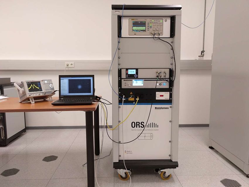
An ultra-stable Laser as an
          optical frequency standard

                                  DIPLOMA THESIS
             submitted in partial fulfillment of the requirements for the degree of

                                  Diplom-Ingenieur
                                               in

                                    Technical Physics

                                               by

                            Thomas Tobias Pronebner, BSc
                                Registration Number 01129159

to the Faculty of Physics
at the TU Wien
Advisor:    Univ.Prof. Dipl.-Phys. Dr.rer.nat. Thorsten Schumm
Assistance: Dr. Michael Matus
            Dr. Jörg Premper

Vienna, 11th July, 2021
                                   Thomas Tobias Pronebner             Thorsten Schumm

                                  Technische Universität Wien
                 A-1040 Wien Karlsplatz 13 Tel. +43-1-58801-0 www.tuwien.ac.at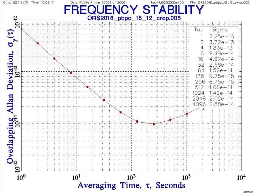
Erklärung zur Verfassung der
                                  Arbeit

Thomas Tobias Pronebner, BSc

Hiermit erkläre ich, dass ich diese Arbeit selbständig verfasst habe, dass ich die verwen-
deten Quellen und Hilfsmittel vollständig angegeben habe und dass ich die Stellen der
Arbeit – einschließlich Tabellen, Karten und Abbildungen –, die anderen Werken oder
dem Internet im Wortlaut oder dem Sinn nach entnommen sind, auf jeden Fall unter
Angabe der Quelle als Entlehnung kenntlich gemacht habe.

Wien, 11. Juli 2021
                                                            Thomas Tobias Pronebner

                                                                                        v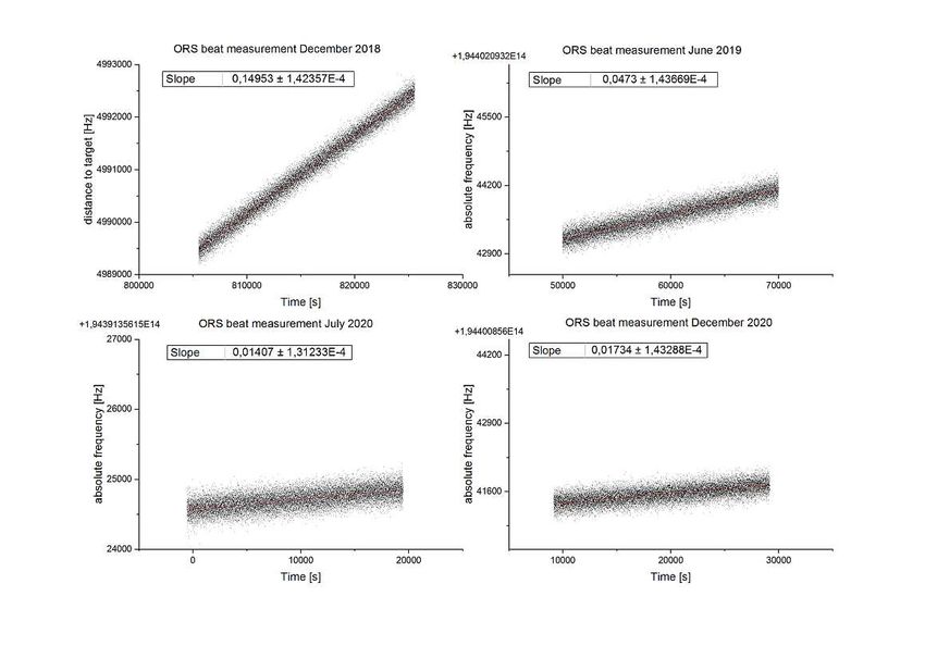
Danksagung

An erster Stelle möchte ich mich bei meinen Eltern bedanken, die mir ein sorgenfreies
Studium ermöglicht haben und mir jederzeit mit Rat und Tat zur Seite gestanden sind.

Des Weiteren möchte ich Thorsten Schumm für die angenehme Betreuung und die un-
heimlich nette Umgangsart danken. Trotz vollen Terminkalenders fand sich immer rasch
ein Termin um meine Fragen oder Sorgen zu klären.

Ein besonderer Dank gebührt dem BEV und meinen Kollegen im BEV, die mich nicht nur
in fachlicher Hinsicht stets hilfsbereit beraten haben. Ich durfte von Michael Matus, Anton
Nießner und Werner Mache sehr viel Wissen aufnehmen und die direkte Zusammenarbeit
mit den Kollegen Georg Zechner, Jörg Premper und Elke Aeikens hat viel zu dieser Arbeit
beigetragen. Auch möchte ich Christina Hofstätter-Mohler und Petra Milota danken, die
mir die Stelle im BEV ermöglicht haben.

Da diese Arbeit im Rahmen des EMPIR Projektes CC4C entstanden ist, hatte ich die
Gelegenheit internationale Partner kennenzulernen. Den Kollegen des ISI in Brünn Ondrej
Cip, Martin Cizek, Lenka Pravdova, Pham Minh Tuan und Jan Hrabina bin ich sehr
dankbar, dass sie mir mit viel Geduld und Freundlichkeit ihr Wissen weiter gegeben
haben.

                                                                                        vii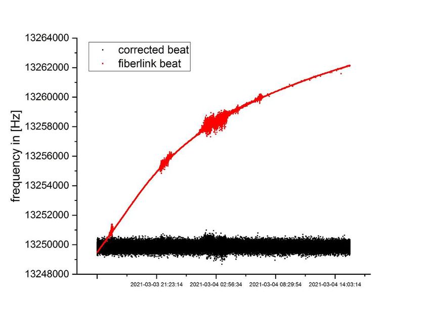
Acknowledgements

First of all, I would like to thank my parents, who made it possible for me to study
carefree and who were always on hand with advice and assistance.

Furthermore, I would like to thank Thorsten Schumm for being my supervisor and the
incredibly friendly manner. Despite his busy schedule, an appointment was always quickly
found to clarify my questions or concerns.

A special thank you goes to the BEV and my colleagues at BEV, who always gave me
helpful advice, and not just in technical matters. I was able to gain a lot of knowledge
from Michael Matus, Anton Nießner and Werner Mache. The direct collaboration with
colleagues Georg Zechner, Jörg Premper and Elke Aeikens has contributed a lot to this
work. I would also like to thank Christina Hofstätter-Mohler and Petra Milota, who
made it possible for me to work at BEV.

Since this thesis was written within the framework of the EMPIR project CC4C, I had the
opportunity to get to know international partners. I am very grateful to the colleagues
at the ISI in Brno, Ondrej Cip, Martin Cizek, Lenka Pravdova, Pham Minh Tuan and
Jan Hrabina, for sharing their knowledge with me with great patience and kindness.

                                                                                      ix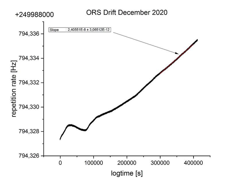
Kurzfassung

Nach mehr als einem halben Jahrhundert als primäres Frequenznormal sind Cäsium-
Atomuhren an die Grenzen der Weiterentwicklung der Präzision gestoßen und eine
Ablösung durch einen präziseres Normal zeichnet sich ab. Die potentiellen Nachfolgernor-
male sind sogenannte optische Uhren, deren Taktgeber eine elektromagnetische Welle im
optischen Teil des Frequenzspektrums ist. Diese optischen Uhren erreichen deutlich höhere
Stabilitäten als Cäsiumstandards (relative Unsicherheit von 10−18 vs. 10−15 ). Einer der
Hauptbestandteile einer solchen Uhr ist ein Laser mit sehr schmaler Linienbreite. Als
ersten Schritt in Richtung des Betriebs einer optischen Uhr in Österreich, wurde im
Zuge des EMPIR Projektes „Coulomb Crystals for Clocks“ (CC4C) vom Bundesamt für
Eich- und Vermessungswesen, kurz BEV, ein solcher Laser beschafft. Des Weiteren wurde
im Rahmen des Projekts zunächst die Schaffung einer Glasfaserverbindung von Wien
nach Brünn evaluiert und im weiteren Verlauf des Projekts auch hergestellt, um eine
Vergleichsmessung des ultra-stabilen Lasers am BEV mit dem Pendant des „Institute for
Scientific Instruments“ (ISI) in Brünn durchführen zu können.
Diese Arbeit beschäftigt sich, nach kurzer Einführung in die Grundlagen, mit der Charak-
terisierung des Driftverhaltens, der Zero-Crossing Temperatur und der Frequenzstabilität
des Lasers und der Erstellung eines Unsicherheitsbudgets. Zur Erstellung der Daten
wurden unter anderem Vergleichsmessungen mit dem ISI in Brünn herangezogen.

                                                                                      xi
Abstract
After more than half a century as primary frequency standard caesium clocks have
exhausted their potential to improve their stability. Therefore, a replacement by a new
standard that is even more precise is imminent. The potential successor standards are
optical clocks, which use energy level transitions that produce electromagnetic waves in
the optical regime of the frequency spectrum. These optical clocks achieve significantly
higher stabilities than cesium standards (relative uncertainty of 10−18 vs. 10−15 ). One of
the main components of such a clock is a laser with a very narrow line width. In the
framework of the EMPIR project “Coulomb Crystals for Clocks” (CC4C), the Federal
Office for Metrology and Surveying (BEV) acquired such a laser as a first step towards
the operation of an optical clock in Austria. Furthermore, as part of the project, the
installation of a fiber optic connection from Vienna to Brno was initially evaluated and,
in the further course of the project, it was also established in order to be able to carry
out a comparison measurement of the ultra-stable laser at the BEV with its counterpart
of the “Institute of Scientific Instruments” (ISI) in Brno.
After a short introduction to the matter, this thesis deals with the characterization of the
laser’s drift behavior, frequency stability, the cavity’s zero-crossing temperature and the
creation of an uncertainty budget. The collected data includes results from comparison
measurements with the ISI in Brno.
xiiiContents
Kurzfassung xi
Abstract xiii
Contents xv
1 Introduction 1
1.1 Time and Frequency . . . . . . . . . . . . . . . . . . . . . . . . . . . . . . 1
1.2 Lasers as frequency standards . . . . . . . . . . . . . . . . . . . . . . . . . 2
1.3 Outline . . . . . . . . . . . . . . . . . . . . . . . . . . . . . . . . . . . . . 3
2 Theoretical Background 5
2.1 Optical Resonator . . . . . . . . . . . . . . . . . . . . . . . . . . . . . . . 5
2.2 Zero-crossing Temperature . . . . . . . . . . . . . . . . . . . . . . . . . . . 10
2.3 Allan Variance . . . . . . . . . . . . . . . . . . . . . . . . . . . . . . . . . 11
2.4 Second Harmonic Generation . . . . . . . . . . . . . . . . . . . . . . . . . 12
3 Ultra-stable Laser System 17
3.1 Laser . . . . . . . . . . . . . . . . . . . . . . . . . . . . . . . . . . . . . . . 17
3.2 Locking Mechanism . . . . . . . . . . . . . . . . . . . . . . . . . . . . . . 17
3.3 Cavity . . . . . . . . . . . . . . . . . . . . . . . . . . . . . . . . . . . . . . 22
4 Fiber Links 25
4.1 Fiber link Brno . . . . . . . . . . . . . . . . . . . . . . . . . . . . . . . . . 25
4.2 Fiber link TU Wien . . . . . . . . . . . . . . . . . . . . . . . . . . . . . . 28
5 Characterisation of the Optical Reference System 31
5.1 Drift Performance . . . . . . . . . . . . . . . . . . . . . . . . . . . . . . . 31
5.2 Frequency stability . . . . . . . . . . . . . . . . . . . . . . . . . . . . . . . 36
5.3 Zero-crossing Temperature Measurement . . . . . . . . . . . . . . . . . . . 38
5.4 Uncertainty Budget . . . . . . . . . . . . . . . . . . . . . . . . . . . . . . 38
6 Conclusion & Outlook 45
xvList of Figures 47 List of Tables 47 Bibliography 49
CHAPTER              1
                                                          Introduction

1.1     Time and Frequency
Time might be, together with length and mass, the most intuitively perceptible physical
quantity. While the other two quantities form the basis for what surrounds us, time
enables the universe to evolve. But also much less philosophically, time is an essential
quantity in everyday business life, social life and science. The unit of time in the Système
international d’unités (SI) is the second and it is defined as:

      “The second, symbol s, is the SI unit of time. It is defined by taking the fixed
      numerical value of the caesium frequency ΔνCs , the unperturbed ground-state
      hyperfine transition frequency of the caesium 133 atom, to be 9 192 631 770
      when expressed in the unit Hz, which is equal to s−1 .” [Gen18]

As the definition suggests, the primary realisation of the second is a caesium clock, in
which Cs atoms travel through a microwave resonator and are excited from the hyperfine
state F = 3 with mF = 0 to the hyperfine state F = 4 with mF = 0 and then detected.
The resonator’s frequency is adjusted to the value where the signal at the detector is at
its maximum. There are several effects like the second-order Doppler shift, gravitational
shift, shifts from magnetic fields, et cetera that shift the energy levels in the atom and,
hence, the transition’s frequency from the unperturbed value. These shifts need to be
mitigated and accounted for. Most of these effects are small or can be well compensated
for the transition that is used in caesium clocks. The caesium clock fulfills its role as
a reliable, stable and affordable realisation of the second very well. Hence, the current
realisation of the second has endured for more than half a century by now (first used as
realisation of the second in 1967). The most sophisticated microwave frequency standard
is the caesium fountain clock, which has a fractional uncertainty of around 10−15 [Rie06].
However, this uncertainty is achieved after averaging over a day. In terms of short-term

                                                                                          1
1. Introduction
stability (averaging time of seconds) there are several frequency standards that provide
better uncertainty than caesium clocks, for instance hydrogen masers and optical clocks.
In recent years the latter have started to surpass caesium clocks not only in short-term
stability (10−13 vs. 10−15 ), but also in long-term stability (10−15 vs. 10−18 ) [MS21].
In a strategy document by the Consultative Committee for Time and Frequency from
2016 a number of milestones were set that have to be achieved in order to warrant a
redefinition of the second [fTF16]. Although some of the milestones, for example in terms
of stability performance and clock comparisons, have been reached, the given earliest
date of redefinition, 2026, seems quite ambitious at this point.
1.2 Lasers as frequency standards
The considerable advantage of lasers over microwave oscillators is their higher frequency.
The optical regime is in the range of several hundred THz, whereas the frequency of
microwaves is in the range of GHz. This advantage is twofold: First, the higher an
ν
oscillator’s frequency, the higher its quality factor Q = Δν , with Δν being the line width.
A high Q is desirable, because it is proportional to the oscillator’s frequency uncertainty.
Second, a high frequency allows faster comparison of two oscillators, hence, resulting in
shorter averaging times for measurements. For example, to reach a fractional uncertainty
of 10−15 with a microwave oscillator takes hours of averaging time, while it only takes
seconds with an optical oscillator.
The typical set-up for a highly stable oscillator in the optical regime consists of a laser
with low phase noise that is locked to an external Fabry-Pérot cavity to further reduce
its phase noise (this topic will be treated in more detail in chapter 3). In an optical
clock such an ultra-stable laser system is used as probing laser that is locked to the
transition frequency of an atom or an ion. In order to keep this transition frequency
as narrow as possible one has to inhibit the movement of the clock atoms/ions (see fig.
1.1). To achieve this suppression of movement, the clock atoms/ions are laser-cooled. To
eliminate the residual motion there are two techniques to trap the atoms/ions, which
divide optical clocks into two types: lattice clocks and single ion clocks. The former uses
lasers, operated in such a way that standing waves occur, which in turn form a lattice of
potential wells. In these potential wells atoms accumulate and are confined to a smaller
space. In single ion clocks, an individual ion is trapped in an electromagnetic field. Both
types have advantages and disadvantages, however, the lattice clocks appear to have a
slight edge because of the high number of emitters that can be trapped.
The obtained optical frequency is too fast for current electronics and cannot be counted
directly. Therefore, a frequency comb generator, which is a mode-locked femtosecond
laser, is used to transfer the frequency from the optical into the RF regime (e.g. 10 MHz)
(for more information see [UHH02]). In figure 1.1 the necessary parts for an optical clock
are summarised in a schematic.
It is important to be able to compare optical oscillators, even over large distances. Espe-
cially, since more and more optical clocks are supposed to contribute to the international
atomic time (TAI). Nowadays most of the contributing clocks are microwave standards
21.3. Outline
and are compared via satellites. However, this comparison technique is not suitable
for the needed accuracy of optical clocks (10−18 ). Phase-coherent fiber links provide a
feasible alternative.
Figure 1.1: Schematic of an ion optical clock setup [GBK+ 21].
1.3 Outline
After a short introduction to the theoretical background on fundamental phenomena
regarding cavities, Allan variance and second harmonic generation in chapter 2, an
overview over the used ultra-stable laser system is given in chapter 3. In chapter 4 the
operated and planned fiber links are described. In chapter 5 the performed measurements
are presented and, finally, in chapter 6 conclusions and an outlook are given.
3CHAPTER 2
Theoretical Background
2.1 Optical Resonator
An optical resonator and the standing waves it produces inside, can be used as a reference
for a laser. In its simplest form is made up of two reflective surfaces. The cavity used in this
work is a hemispherical resonator, i.e. a resonator with one plane mirror and one concave
mirror. If we look at an optical resonator from the idealised perspective of ray optics,
the problem is quite simple, and the basic principles can be clearly demonstrated. The
c
smallest possible mode in the resonator with length L has a frequency of f = 2L (see fig.
2.1a), because only standing waves are reasonably stable over time. The electromagnetic
wave between the mirrors will gradually suffer energy losses due to imperfect reflectivity
of the mirrors (fig. 2.1c). Therefore, the mode will decay exponentially with some rate
1
τ , which is directly proportional to the losses and approximately the mode’s linewidth
Δf ≈ τ1 (fig. 2.1b). If there were no losses at all in the resonator, the contribution to the
mode’s linewidth would be zero and the frequency would resemble a delta function. So,
the lower the losses the narrower the linewidth. One can achieve a narrower linewidth
by either compensating the losses with a gain medium, which is done in lasers, or by
improving the mirror’s reflectivity. The latter is done in external cavities, however, there
is a certain limit to maximising the reflectivity R, because light has to be injected into
the resonator, which is not possible if R = 1 and, hence, the transmission T equals zero.
An optical resonator can accommodate many modes, as long as their frequencies meet
the following boundary condition:
2L
λn = , resp. (2.1)
n
c
fn = n · , (2.2)
2L
52. Theoretical Background
(a) Smallest stable longitudinal mode between
two mirrors that are a distance of L apart. Its
wavelength is twice the resonator’s length.
(b) (c)
Figure 2.1: Due to imperfect reflectivity of the resonator’s mirrors the electromagnetic
waves suffer power losses and decays exponentially with a rate of τ1 , which can be seen in
(c). The resulting linewidth corresponds to approximately the rate of decay (b).
with n being the mode number (see fig. 2.2). Because the resonator only allows certain,
c
discrete longitudinal modes with finite linewidth, there is a spacing of 2L between the
modes. This distance is called the free spectral range (FSR). Beside longitudinal modes
there are also transverse modes that have to be taken into account. Usually one wants to
have a single spot with a Gaussian power distribution, which corresponds to the TEM00
mode. This mode is favourable, because it confines all of the power in one area, in
contrast to all higher modes that consist of several spots (fig. 2.3a). These modes have a
different optical path in the cavity, therefore their frequency is slightly different from
that of the TEM00 mode. For reference see the excellent lectures of Prof. Shaoul Ezekiel
[Sha08].
62.1. Optical Resonator
Figure 2.2: Frequency picture of several modes in a resonator equidistantly spaced by
the free spectral range.
For optical resonators that are used as an external cavity, in order to reduce the linewidth
of a laser, the reflectivity/transmission is an important quantity. In this case the cavity
can be described as a Fabry-Perot interferometer, which consists of two plane mirrors
between which the light waves bounce back and forth and pass the cavity only if they
are in resonance with the interferometer, i.e. fulfill condition (2.1). The transmission of
(a) (b)
Figure 2.3: (a) Transverse laser modes in a cavity with circular mirrors [Wik08]. (b)
Picture of the TEM00 mode of BEV’s ultra-stable laser system.
72. Theoretical Background
a Fabry-Perot interferometer is given by the following formula:
1
T = (2.3)
1 + F sin2 ( 2δ )
where
4r2
F = (2.4)
1 − r4
is the coefficient of finesse which is proportional to the finesse and r is the electric field
reflectivity. δ describes the phase difference between two rays in the resonator
4πnL
δ= cos(θ). (2.5)
λ
In fig. 2.4 a Fabry-Perot cavity’s transmission is plotted as a function of δ for two different
values of reflectivity. The higher the reflectivty of the mirrors, the higher is the cavity’s
finesse and, hence, the narrower are the transmitted peaks. The finesse describes the
ratio of the FSR to the linewidth:
fFSR
Finesse = . (2.6)
Δf
82.1. Optical Resonator
Figure 2.4: A Fabry-Perot cavity’s transmission as a function of phase difference δ for a
power reflectivity of 0.75 and 0.95. These values roughly correspond to finesse values of 5
respectively 30. The cavity used in the ORS has a finesse of 320000 and the peak profile
is very close to a delta-function. The picture was created with a Matlab script based on
the code in this reference [Sul15].
92. Theoretical Background
2.2 Zero-crossing Temperature
As mentioned previously, cavities can be used to lock a laser’s frequency to the cavity’s
resonance frequency. The resonance frequency changes with cavity length, i.e. thermal
expansion. So for a good lock performance, the cavity’s length changes due to temperature
have to be kept at a minimum. Certain types of materials have a temperature, where
their coefficient of thermal expansion (CTE) crosses zero; e.g. water and also ultra low
expansion (ULE) glass. Below this point the material contracts when heated and above
this point the material expands when heated. When a cavity is kept at this “zero-crossing
temperature” its length changes due to thermal expansion are the smallest.
(a) (b)
Figure 2.5: Graphs of the CTE and density of water. Because of the CTE’s zero crossing
there is a maximum in the density plot. In section 5.3 we will see this extremum in a
frequency plot, due to the relationship of a cavity’s length and its modes’ frequencies.
ULE glass has a CTE of 3 × 10⁻⁸ K−1 [Cor]. For a cavity that is 12.1 cm long, this
means that a change of 1 Kelvin results in a change in cavity length of 3.6 nm. For a
wavelength of 1550 nm this translates to a change of 0.05 pm in wavelength respectively
roughly 6 MHz in frequency.
102.3. Allan Variance
2.3 Allan Variance
The Allan variance, or its root the Allan deviation, is used as a measure for the stability
of an oscillator. It is determined by comparing two oscillators, where one of them usually
acts as a reference to which the other oscillator is compared. It is defined as:
2
2
1 2 1
σy2 (τ ) = ȳi − ȳj = (ȳ2 − ȳ1 )2 , (2.7)
i=1
2 j=1 2
where
ti +τ
ȳi = y(t)dt, (2.8)
ti
with τ being the measurement time and
Δν(t)
y(t) = (2.9)
ν0
being the fractional frequency deviation. The main difference of the Allan deviation in
comparison to the standard deviation is that it describes the difference between adjacent
frequency values instead of the difference of a frequency value to the mean. For reference
see [Rie06]. The Allan deviation is usually given as a plot for several values of τ as shown
in fig. 5.6a. From the slope of the Allan plot one can obtain information about the
different kinds of noise on the signal. There are several versions of the Allan deviation
that serve different purposes, e.g. the so-called “modified Allan deviation” where white
phase modulation and flicker phase modulation have a different slope in the Allan plot
and, hence, can be distinguished, which is not possible in the original Allan deviation.
112. Theoretical Background
2.4 Second Harmonic Generation
In order to link BEV’s traceable frequency source to the experiments at ATI, the
transferred laser light has to be frequency doubled (see section 4.2). This is done with a
technique called second harmonic generation. Second harmonic generation is a process
that uses the non-linear properties of a material’s polarisation function
P (E) = 0 χ(1) E + χ(2) E 2 + χ(3) E 3 + ... (2.10)
to generate light with double the frequency with respect to the incoming light. Looking
at the quadratic term in (2.10)
3
(2)
Pi = χi,j,k Ej Ek , i, j, k = 1, 2, 3 (2.11)
j,k=1
and considering a superposition of two waves E1 and E2 , the following product terms
Ei Ej will arise:
2
(E1 + E2 ) = E01 cos2 ω1 t + 2E01 E02 cos ω1 t cos ω2 t + E02
2
cos ω2 t
2
E01 E2
= (1 − cos 2ω1 t) + 02 (1 − cos 2ω2 t) (2.12)
2 2
+ E01 E02 [cos(ω1 − ω2 )t − cos(ω1 + ω2 )t] .
In equation (2.12) terms with the doubled frequencies 2ω1 , 2ω2 and the sum and difference
frequency occur. In case that ν1 = ν2 , one speaks of second harmonic generation, where
two photons of frequency ν combine to one photon with the doubled frequency ν3 = 2ν .
This will be the relevant process in section 4.2.
One important factor that has to be considered in SHG is phase matching. The polarisa-
tion wave created in the crystal by the incident light (ωfund ), travels through the crystal
with the same velocity as the incident light. This velocity is determined by the index of
refraction n(ωfund ). The value of the refractive index generally depends on the frequency
of the light. The polarisation wave creates light with two times the frequency of the
c
fundamental light ωharm = 2ωfund . Hence, its phase velocity v = n(ωharm ) will be different.
The phase of already created second harmonic light and newly created second harmonic
light, which follows the phase of the fundamental light, will sinusoidally fall in and out of
phase. After a distance called the coherence length the frequency doubled waves are in
phase they will positively interfere and after twice this distance they are out of phase
and will annihilate. Hence, one has to match the phase of ideally all created photons to
receive the maximum yield. One way of realising this is so-called critical phase matching,
where one uses a uniaxially birefringent crystal, which has two eigenmodes of polarisation,
called the ordinary and extraordinary beam. The refractive index of the ordinary beam
no is isotropic. The extraordinary beam’s refractive index ne , however, is dependent on
the incident angle of light. If one guides light through the crystal at a critical angle, the
refractive index of the frequency doubled extraordinary beam ne (2ω ) will be equal to
122.4. Second Harmonic Generation
the refractive index of the ordinary, fundamental wave no (ω) (see fig. 2.6a). With both
refractive indices being the same, the phase of the fundamental wave and the second
harmonic wave will match along the crystal. The electric field of the second harmonic
will increase linearly and its power quadratically. A downside to this technique is that
the phase matching condition can only be realised for a limited range of frequencies.
With a method called quasi phase matching, one can extend this range of frequencies.
Here, the crystal’s polarisation is periodically modulated in such a way that its direction
changes every multiple integer of the coherence length. So, after each distance where the
second harmonic reaches its plateau of positive interference, and the waves would start
to annihilate, the change of direction in polarisation introduces a phase shift of π and,
hence, back into the range of positive interference. For reference see [Rie06].
(a)
(b)
Figure 2.6: (a) Magnitude of the refractive index as a function of angle of incident. The
refractive index of the ordinary beam is isotropic and therefore a circle in this graph.
The extraordinary beam’s refractive index depends on the angle of incident θ and forms
an ellipse. If the angle of incidence coincides with the optical axes, the refractive indices
are the same for both beams. The crossing point between the ellipse of no (2ω ) and the
circle of ne (ω) defines the phase matching condition no (2ω) = ne (ω). [Rie06]
(b) This picture shows the second harmonic’s power function without phase matching in
“a”, critical phase matching in “b” and quasi phase matching in “c”. [Rie06]
2.4.1 Optical Arrangement
The TEM00 mode of a laser has a Gaussian beam profile, which means that its amplitude
envelope is given by a Gaussian function. In contrast to ideal ray optics, a Gaussian
beam cannot be focused to a infinitely small spot, but only to a finite cross section with
a certain beam waist w0 . The beam width as a function of propagated distance z is given
as
2
z
w(z) = w0 1 + , (2.13)
zr
132. Theoretical Background
where
πw02 n
zr = (2.14)
λ
is the Rayleigh length. In section 4.2 a periodically poled Lithium Niobate (PPLN)
crystal is used for second harmonic generation. For optimal conversion in the PPLN
crystal the laser light has to be focused into the center of the crystal. Furthermore, the
ratio of the length of the crystal to the confocal parameter (b = 2zr ) has to be 2.84
[BK68]. When choosing the focusing lens, one has to consider the different refraction
indices of air and the crystal. The procedure for calculating the focal length of the lens
and the required beam width after the collimator was to first calculate b from
l
= 2.84, (2.15)
b
which is 14.1 mm for a crystal length of 40 mm. With (2.14) one gets a beam waist w0 of
40.3 µm. With (2.13) one can calculate the beam width at the edge of the PPLN crystal
and consequently the beam width at the focusing lens. For example with a lens with a
focal length of 50 mm, the beam width at the lens and, hence, also after the collimator
decoupling the light from the fiber, is around 0.5 mm, which corresponds to a beam
diameter of 1 mm.
An overview of this topic can be found in [Edm] and [Cov].
Figure 2.7: The relevant parts of the optical arrangement for second harmonic generation
with a PPLN crystal. Half the crystal is depicted in green and the focusing lens in
blue. The ratio of the length of the crystal to the confocal parameter is given by [BK68].
From the confocal parameter one can calculate a suitable focal length - beam diameter
combination. The schematic was drawn with the programme OpticalRayTracer [Lut17].
142.4. Second Harmonic Generation
(a) (b) (c)
(d)
Figure 2.8: Pictures (a) to (c) show a Gaussian beam profile diverging while propagating
in z direction. In (d) the smallest cross section is marked as w0 and
√ is called beam waist.
After the Rayleigh length zr the beam width increases to wr = 2w0 . The parameter
b = 2zr is called the confocal parameter.
15CHAPTER 3
Ultra-stable Laser System
The ultra-stable laser is a so-called “Optical Reference System 1500” (ORS1500) made by
Menlo Systems [Mena]. The ORS contains a RIO Planex Laser Diode that is stabilized
with an external cavity (length = 12.1 cm) by a Pound-Drever-Hall (PDH) locking system
(fig. 3.1). It operates at a wavelength of 1542.14 nm, which corresponds to a frequency
of roughly 194.4 THz. This wavelength was chosen in order to match the ITU-T DWDM
channel 44 [ITU20] for optimal transfer conditions via glass fiber. The ORS is very
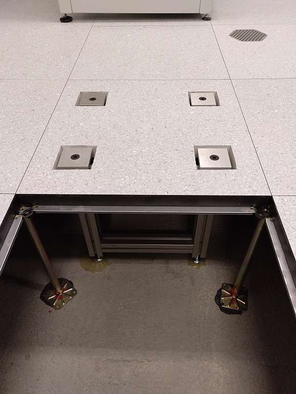
sensitive to vibration and temperature fluctuations, hence, the cavity and the optics are
in a temperature stabilised chamber. This chamber rests on an aluminium frame that
was built to protect the ORS from floor vibrations (fig. 3.2). Additionally, the optics and
the cavity are set up on an active vibration isolation platform. The surrounding rack
with the electronics is supported by a separate set of wheels.
3.1 Laser
The laser diode already has a fairly narrow linewidth of 2.8 kHz (Lorentzian FWHM).
However, for clock operation the desired linewidth is in the sub-Hertz range, so the laser
is locked to an external cavity to suppress the noise level even further, resulting in a
sub-Hertz linewidth. The output power of the RIO Planex is 20 mW and the output
power of the stabilised light is 8 mW.
3.2 Locking Mechanism
The Pound-Drever-Hall Locking technique creates an error signal by mixing the beat note
from a laser’s reflection off a cavity and a side-band that was modulated onto the laser’s
light with an EOM and an RF signal from a local oscillator. This error signal is fed to the
laser’s actuators1 via a loop filter to keep the laser’s frequency as close to the resonance
1
The laser current acts as the fast actuator and the laser temperature control is the slow actuator.
173. Ultra-stable Laser System
Figure 3.1: Picture of the ORS shortly after its arrival in 2018.
of the external cavity as possible. The main advantage of this locking mechanism is that
the error signal generation is theoretically independent of power fluctuations produced
by the laser.
The following discussion of the PDH locking scheme follows along the derivation in the
introductory paper by Eric Black [Bla00]. As seen in fig. 3.3 a part of the laser’s output
is guided through an electro-optic modulator (EOM), where the laser light is phase
modulated with an RF frequency Ωm :
Einc = E0 ei(ωt+β sin(Ωm t)) . (3.1)
Due to the birefringence of the crystal in the EOM, care must be taken that the
polarization of the input beam and the principal axes of the crystal are aligned. A
misalignment will give rise to a residual amplitude modulation (RAM), which will be
discussed below in section “Residual Amplitude Modulation - RAM”. Equation (3.1) can
183.2. Locking Mechanism
Figure 3.2: Aluminium pedestal to decouple the ORS from vibrations on the laboratory’s
floor.
Figure 3.3: Schematic of the ORS1500 PDH locking system. [Men18]
be expressed with Bessel functions as
Einc ≈ [J0 (β) + 2iJ1 (β) sin(Ωm t)] eiωt (3.2)
= E0 J0 (β)eiωt + J1 (β)e(ω+Ωm )t − J1 (β)e(ω−Ωm )t . (3.3)
So the result is the original frequency of the laser at the center flanked by a sideband
above and below at a distance of the modulation frequency Ωm . The modulated frequency
193. Ultra-stable Laser System
passes a polarising beam splitter (PBS) and a quarter wave plate before reaching the
cavity. The reflected light from the cavity will pass the quarter wave plate twice, which
effectively let’s it act as a half wave plate that rotates the polarisation in such a way
that the light is reflected at the PBS towards the photo detector. Almost all of the total
power of the incident beam P0 = E02 is distributed to the carrier PC = J02 (β )P0 and
each of the first order sidebands PS = J12 (β)P0 . In total
PC + 2PS ≈ P0 . (3.4)
With the reflection coefficient F (ω) the reflected power is
Pref = PC |F (ω)|2 + PS |F (ω + Ωm )|2 + |F (ω − Ωm )|2
+ 2 PC PS {Re [F (ω)F ∗ (ω + Ωm ) − F ∗ (ω)F (ω − Ωm )] cos(Ωm t) (3.5)
+Im [F (ω)F ∗ (ω + Ωm ) − F ∗ (ω)F (ω − Ωm )] sin(Ωm t)}
+ (2Ωm terms).
The detector sees terms of constant power, two terms that oscillate with the mod-
ulation frequency Ωm , which will be the ones of interest, and terms with 2Ωm . In
case Ωm ωFSR , F (ω ± Ωm ) is −1 because the sidebands are totally reflected when
the laser is near or in resonance with the external cavity. Hence, the expression
[F (ω)F ∗ (ω + Ωm ) − F ∗ (ω)F (ω − Ωm )] is purely imaginary and only the sinus in (3.5)
survives. The output of the photo diode is mixed with a radio frequency of Ωm from a
local oscillator2 resulting in a product of two sines with either the sum or the difference
frequency.
1
sin(Ωt) sin(Ω t) = cos (Ω − Ω )t − cos (Ω + Ω )t . (3.6)
2
Since both inputs, the local oscillator (Ω ) and the laser (Ω), have contributions with the
same frequency Ωm this product will be a DC signal (cos(0)), which is isolated with a
low-pass filter. The result is an error signal (fig. 3.4)
4 δω
≈− PC PS (3.7)
π δν
where δν is the cavity’s linewidth and δω is the deviation of the laser frequency from
the cavity’s resonance. Close to the resonance the error signal can be approximated as a
linear function
= Dδf (3.8)
with
√
8 PC PS
D=− . (3.9)
δν
2
The signal coming from the local oscillator is phase shifted to compensate unequal delays on the
two signal paths.
203.2. Locking Mechanism
Figure 3.4: PDH error signal.
The steeper the slope D, the better the lock performance. D, on one hand, depends on
the cavity linewidth and on the other hand on the ratio of the power in the sideband
to the power in the carrier. As stated in [Rie06] the optimal ratio is PPCS = 0.42 which
corresponds to a modulation depth3 β of 1.08. The error signal is fed to the fast actuator
(laser current) and the slow actuator (laser temperature) via an PIID controller. With
this locking technique the laser’s linewidth is slimmed down from the kHz range to a
sub-Hertz linewidth.
3.2.1 Residual Amplitude Modulation - RAM
As mentioned earlier, in principle, the PDH locking scheme is not susceptible to error
signal noise due to fluctuations in laser amplitude, as it is locked to a minimum of the
reflected power. However, temperature fluctuations of the EOM can give rise to RAM
that oscillates with the modulation frequency. Therefore, this RAM passes the mixer
and contributes to the error signal, resulting in an offset to the actual minimum of
reflected power. It originates from the birefringent properties of the electro-optic crystal
in the EOM. If the polarisation of the laser light is not aligned with one of the principle
3
The modulation depth is a measure that describes how much the modulated variable varies around
the unmodulated value.
213. Ultra-stable Laser System
axes, the polarization components experience different phase shifts that are modulated
with the modulation frequency. The PBS after the EOM will then convert the phase
modulation into an amplitude modulation. In practice it is very difficult to achieve
a perfect alignment due to vibrations and temperature fluctuations. There are some
techniques to suppress RAM ([ZMB+ 14]), e.g. by taking two crystals that are rotated in
such way that the phase shifts, caused by the crystals due to polarization, cancel each
other or actively suppressing the RAM with a control loop that modifies the modulation
frequency.
3.3 Cavity
The external high-finesse (320000) cavity is made from ultra low expansion glass (ULE)
and has a length of 12.1 cm which roughly corresponds to a FSR of 1.24 GHz. The
cavity is kept at a steady temperature with a thermoelectric cooler (peltier element).
As mentioned in section “Locking Mechanism” the cavity is the dominating source of
instability in the frequency. Hence, it has to be protected from environmental influences.
Therefore, the cavity is within a vacuum chamber with a pressure of 8 × 10⁻⁹ mbar to
suppress vibrations and heat transfer. The working vacuum pressure is maintained with
an ion getter pump. To minimise the contact surface, the cavity rests on four small
rubber balls. In order to keep the influence of thermal expansion at minimum, the cavity
is kept at the so-called zero-crossing temperature (section 2.2). However, no matter how
well a cavity is isolated, there will always be a continuous change in length due to aging
- the amorphous material, the cavity is made of, shrinks over time. This results in a
(nearly) linear drift in frequency. Furthermore, this drift decreases over long periods of
time, as the cavity ages (see section 5.1).
223.3. Cavity
Figure 3.5: The ORS’s cavity and its vacuum container [Menb].
23CHAPTER 4
Fiber Links
Current atomic clocks, based on microwave transitions, are compared via satellites. This
comparison technique, however, can only achieve a fractional frequency uncertainty of the
order of 10−15 ([Rie06], chapter 12.5). Compared to the fractional uncertainties of optical
clocks of 10−18 , current GPS measurement techniques are not an adequate technology
for comparisons of optical clocks. A suitable alternative are phase-coherent fiber links.
4.1 Fiber link Brno
The stability of ultra stable lasers after averaging times of a few to several 100 seconds is
at least two orders of magnitude better than RF oscillators. Therefore, it is not possible
to measure the full stability potential of the ORS with a comb that is locked with RF
reference signals. To further investigate the short term stability of the ORS it has to be
compared with another ultra stable laser. As part of the EMPIR research project CC4C
the ORS was compared to an ultra stable laser at the ISI in Brno. The ISI and BEV were
connected via glass fiber. The used fiber is kept free from any other (commercial) traffic
and is therefore called a “dark fiber”. To compensate for the losses along the 240 km long
fiber bi-directional amplifiers have to be used. For a meaningful comparison the fiber has
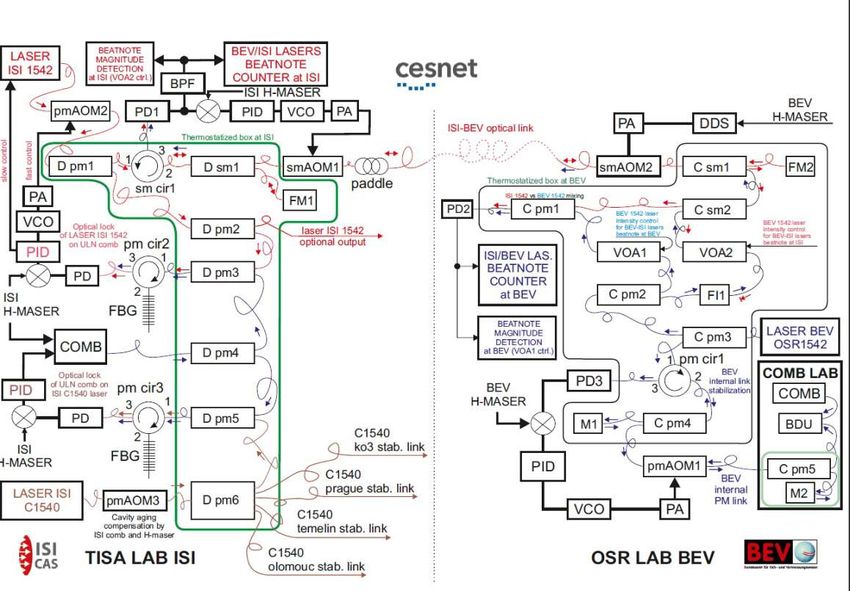
to be phase-stabilised. A schematic picture of the link can be seen in figure 4.1. The
two ultra stable lasers on both sides can be used as either master or slave laser in this
configuration. As soon as the phase stabilisation of the link works satisfactory this will
allow a transfer of information from and to both sides of the link via the ultra stable
lasers. For example a comparison of the two H-masers is in preparation. The principle
of the phase stabilisation is the same as in this paper [MJYH94]. As stated before, this
link can work in both directions, so, for this discussion the Czech laser is declared as the
master laser and the ORS as the slave laser. In the schematic the laser that is transferred
from Brno to Vienna is called “Laser ISI 1542”. It is a Koheras Basik Laser with narrow
linewidth that is locked to a frequency comb, which is in turn locked to the ultra stable
254. Fiber Links
Figure 4.1: Schematic of the fiberlink and its stabilisation [Cip19].
laser at Brno (“Laser ISI C1540”). This has to be done because the ORS in Vienna is at
1542 nm while the ultra stable laser in Brno is at 1540 nm. This gap in wavelength is too
large for a beating measurement (≈ 300 GHz). Therefore the stability of the “Laser ISI
C1540” is transferred to the “Laser ISI 1542” via a lock to the frequency comb. The laser
“Laser ISI 1542” passes a circulator “sm cir1” from port 1 to port 2 and a splitter “D
sm1” before going through an AOM “smAOM1” that is driven with an radio frequency
of 80 MHz. This AOM is the actuator for the control loop that compensates the phase
noise collected along the fiber. The signal then enters the fiber link to Vienna. In the
ORS laboratory the light first passes a manual fiber polarisation controller (paddels).
Along the link the temperature around the fiber fluctuates and with it the polarisation
of the light. The paddles help to rotate the polarisation of the signal from Brno to the
desired angle for the measurement done in Vienna. Next in line is the second AOM
“smAOM2” which modulates a constant 40 MHz onto the signal. This is done to mark
the reflection at the end of the fiber link1 and, thus, the correct signal for the beating
measurement back in Brno can be identified. After the AOM the signal is split. The
majority of the signal is directed to the experiments at BEV and the rest is reflected back
1
The link consists of several connected fibers. On any of those connections, or parts in the link or
sharp bends there could be (strong) reflections. These could be mistaken as the reflection from the end
of the fiber and lead to wrong compensations of the control loop.
264.1. Fiber link Brno
into the link with a Faraday mirror “FM2”. The light passes the two AOMs again and
has now collected a total frequency shift of 240 MHz. In the splitter “D sm1” the light
from the link is combined with the reflected light from mirror “FM1”. The combined light
passes the circulator “sm cir1” from port 2 to port 3. The photodiode “PD1” detects
the beat-note between the light from mirror “FM1” and from the round-trip along the
fiber link. This beat is mixed with an RF signal from ISI’s H-maser to generate an error
signal for a phase-locked loop (PLL). The PLL compensates the noise collected along the
fiber link by shifting the transferred laser light with the AOM in such a way that the
phase relation between the beat-note and the (multiplied) RF signal from the H-maser
remains constant.
At this point in time the fiber link is active and the link stabilisation is working, as can
be seen in figure 4.2. The settings of the compensation loop still have to be fine tuned for
optimal lock performance. Measurements of the beat-note between the ORS and the laser
signal from Brno were made to analyse the phase noise. These beating measurements
were also used in sections 5.2 and 5.4 to investigate the ORS’ frequency stability.
Figure 4.2: Phase noise reduction due to link stabilisation [CPH+ 21]. The green line
represents the profile of a laser with 1 Hz linewidth.
274. Fiber Links
4.2 Fiber link TU Wien
As part of the EMPIR project CC4C a fiber connection from the BEV to the “Atominstitut”
(ATI) of the TU Wien was established. This fiber connection makes it possible to trace
frequency standards at the ATI to the national frequency standard at BEV. This
metrological traceability is realised by transferring the ORS signal to the ATI via a
phase-stabilised dark fiber as described in the previous section 4.1. In contrast to the
connection between the ISI and the BEV bi-directional amplifiers are not needed, because
the distance is a lot shorter. Instead, at the ATI a very stable laser (Koheras Basik by
NKT) is phase-locked to the ORS signal from the glass fiber. This offers a relatively
cheap opportunity to refresh the stabilised signal from a few µW to 40 mW. The locked
Koheras Basik is then frequency doubled with a second harmonic generation (SHG)
crystal. The laser light at 771 nm is then used as a traceable reference for experiments
at the ATI.
The locking electronics are kindly provided by ISI and implemented in the same chassis
that holds the electronics for BEV’s side of the ISI-BEV link. For the frequency doubling
via second harmonic generation a Magnesium-Doped Periodically Poled Lithium Niobate
(MgO:PPLN) crystal is used. The crystal is 40 mm long and has a working temperature
of 50 ◦C or 120 ◦C depending on which grating on the crystal is used. The yield of the
SHG process is strongly dependent on crystal temperature, because the temperature
dependency of the refractive index has to be considered for phase matching as discussed
in section 2.4. Already half a degree Celsius off the optimal temperature decreases
the conversion efficiency noticeably. Consequently, the crystal is kept at a stabilised,
steady temperature (±0.01 ◦C) inside an oven. Another important factor for conversion
efficiency is polarisation. Therefore, a half-wave plate is integrated in the setup. The
setup is depicted in figure 4.3. The Koheras Basik’s light is coupled out of the fiber
with a collimator, which determines the light’s beam diameter. The beam passes the
aforementioned half wave plate, before reaching the first plano-convex lens (L1) for
focusing the beam into the center of the PPLN crystal. This process is discussed in
section 2.4.1. After the crystal another plano-convex lens (L2) re-collimates the beam
and the frequency doubled light is seperated from the fundamental light with a dichroic
mirror (M1). The 771 nm light is transferred to the experiments at ATI and the 1542 nm
light is used to lock the fibre laser to the ORS.
284.2. Fiber link TU Wien
Figure 4.3: Schematic of the second harmonic generation setup.
29CHAPTER 5
Characterisation of the Optical
Reference System
5.1 Drift Performance
The cavity’s drift was measured by a beat-note measurement between a frequency comb
and the ORS output. Shortly after delivery, the linear drift was around 150 mHz/s but
decreased towards 70 mHz/s over the course of a year. The linear drift has decreased
ever since to 20 mHz/s at present, which corresponds to 1.73 kHz/d.
Setup
For the measurement the output of the ORS and the fundamental output of the Ultra
low noise (ULN) comb were connected to a “beat detection unit” (BDU) via fibers.
The BDU’s signal was counted with an FXE frequency counter by K+K Messtechnik
[KK]. The raw data provided by the comb’s software was processed by a program called
“TestComb” [Mic16] by Michael Matus. The program “TestComb” calculates the laser’s
absolute frequency after the user provides 3 parameters: the signs of the repetition
rate and the carrier envelope offset frequency (foff ), as well as the mode number of the
comb tooth that is closest to the cw laser. The repetition rate and foff are retrieved
automatically from the measurement’s data file. The visualisation of the processed data
was done with the software Origin.
Results
Effectively, the drift data is continuously acquired. So in this section only a selection
of data sets is presented as examples to show the cavity’s drift performance over time.
Figure 5.2 shows four measurements, each over the period of 20000 seconds, which are
roughly 5.5 hours. This measurement duration was selected because it is a realistic time
315. Characterisation of the Optical Reference System
Figure 5.1: Schematic of the beat measurement.1
date linear drift standard deviation
December 2018 149.53 mHz/s 1.424 × 10⁻¹ mHz/s
June 2019 47.3 mHz/s 1.437 × 10⁻¹ mHz/s
July 2020 14.07 mHz/s 1.312 × 10⁻¹ mHz/s
December 2020 17.34 mHz/s 1.433 × 10⁻¹ mHz/s
Table 5.1: Exemplary results from drift measurements.
frame for real comparison measurements. This is due to the fact that after this period
the stability of the free running ORS starts to deteriorate significantly, as can be seen in
section 5.2. The results are summarised in table 5.1.
It is worth mentioning that the linear drift is not as well behaved as it appears from these
5.5 hour data sets. As one can see in figure 5.3 there are steps in the ORS’s frequency
curve. Most of these steps can be directly linked to spikes in the room temperature. This
is because the air-conditioning system in the laboratory is not ideal for our application.
Some adjustments have already been made and the room temperature stability has
improved. However, for reliable measurements the laboratory must not be entered and
1
The schematic was made in Inkscape using the ComponentLibrary [Ale]
325.1. Drift Performance
Figure 5.2: Decline of linear drift over time from 150 mHz/s at the time of delivery to
below 20 mHz/s at present.
the measurement is controlled remotely. The driving factor for the temperature dependent
frequency fluctuations is RAM as discussed in 3.2.1 which introduces an offset to the
error signal and shifts the locking point. The laser is then locked to a slightly different
frequency.
Also, the linear drift’s magnitude changes with temperature around the CTE’s zero-
crossing temperature [LJW+ 18]. It is the lowest at the zero-crossing temperature.
It is possible to compensate the ORS’ drift by shifting its output with an AOM. The
simplest countermeasure would be to change the AOM’s RF frequency source at the same
rate as the linear drift of the ORS (e.g. 18 mHz/s). This would roughly suppress the
overall linear drift, however, as can be seen in figure 5.3, the linear drift rate is not always
constant. Moreover, small, non-linear changes to the frequency would not be compensated.
There is a more sophisticated way that combines the short-term stability of an ultra-stable
laser with the long-term stability of a H-maser. This can be done by optically locking
a frequency comb to the ORS. More precisely, with a beating measurement between
the ORS and the comb a comb tooth is kept at a constant (frequency) distance to the
ultra-stable laser source with a PLL. This locks the repetition rate frep of the frequency
comb generator to the ORS. The carrier envelope offset foff , however, stays locked to the
335. Characterisation of the Optical Reference System
Figure 5.3: Nonlinearities of the ORS’s drift. In this case the drift data was collected
by measuring the ULN comb’s repetition rate which was locked to the ORS. The shown
repetition rate drift corresponds to a drift of the ORS of 18.706 mHz/s.
RF reference, which is in this case a maser. Although the maser’s stability at 1 second
averaging time is roughly two orders of magnitude worse than the laser, there will still be
a considerable improvement in the frequency comb’s overall short-term stability. Because,
when one takes a look at the comb equation
fLaser = m · frep ± foff ± fbeat (5.1)
one can see that the repetition frequency contributes to the laser frequency with an
integer factor m, which is the mode number and of the order of 105 . So the instability
of foff is negligible compared to frep . A disadvantage of locking the repetition rate to a
free running optical reference is that frep will now drift at the same rate as the laser. To
prevent this, one can introduce an AOM into the connection between the ORS and the
photodiode that measures the beat. The RF frequency that drives the AOM is varied in
such a way that the repetition rate stays at a constant value. This constant frequency
value and the AOM driver’s frequency are provided by Direct Digital Synthesizers (DDS)
345.1. Drift Performance
Figure 5.4: In this figure the beat between the ISI’s laser and the ORS is shown in red.
The black curve is the beat note but corrected for the ORS’s drift. This signal is noisier,
as the ORS’s drift was determined with a comb measurement. This comb measurement,
in contrast to the beating measurement, is not processed with a tracking oscillator. One
can see that the laser signal from the ISI is not significantly drifting, even though it is
locked to a cavity stabilised laser.
that are referenced to the maser. As a consequence, the ORS signal after the AOM will
have both the short-term stability of a cavity stabilised laser and the long-term stability
of a microwave standard - the best of both worlds. This also means that the output
of the compensated ORS no longer shows a drift, linear or non-linear. However, the
quality of the compensation depends on how well the control loop is tuned. For example
the compensated laser of our colleagues of ISI demonstrates a nicely behaved, constant
frequency2 (see fig 5.4). Such a drift compensation loop is planned for the near future
and will greatly improve the ORS’ stability performance.
2
Technically, the laser that was transmitted to and measured at BEV is not the stabilised laser
reference. But this transmitted laser is locked to the frequency comb at ISI that is optically locked to
their drift compensated reference laser. Hence, a drift in their reference laser would translate into a drift
of the transmitted laser.
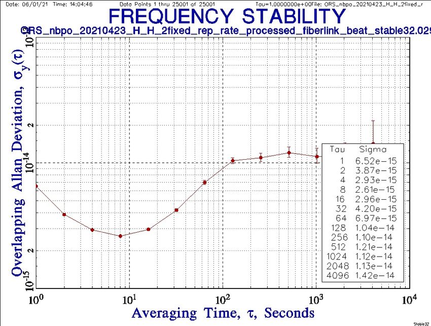
355. Characterisation of the Optical Reference System
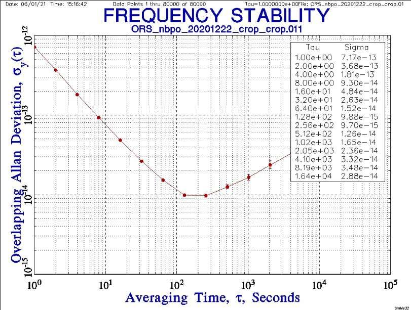
Figure 5.5: ORS fractional frequency stability measured with a beating measurement of
two ultra stable lasers.
5.2 Frequency stability
The ORS’ frequency stability was measured with a beating measurement and expressed
in terms of overlapping allan deviation. The measurements were done with the H-maser
referenced frequency comb as the reference oscillator as well as an ultra-stable laser from
ISI as the reference oscillator. For the determination of the overlapping allan deviation
the ORS’s drift was removed via linear regression. Otherwise the linear drift from cavity
aging would overshadow the frequency fluctuations from other sources. The drift rates in
figures 5.6a and 5.6b differed by about 100 mHz/s, however, after removal of the linear
drift the underlying frequency stability is the same in both cases. A comparison with
figure 5.5 shows that the frequency stability measured with the frequency comb does
not represent the stability of the laser but rather that of the H-maser, especially for
averaging times up to 1 × 10² seconds. After this time period the non-linear parts of the
drift become noticeable and the laser’s stability deteriorates. The measurement shown
in figure 5.5 can still be improved, but considering that the two measured lasers are
more than 100 km apart, these preliminary results are satisfactory. Improvements in lock
performance will move the measured frequency stability closer to the actual frequency
stability of the ORS which is in the low 1 × 10⁻¹⁵ range.
365.2. Frequency stability
(a)
(b)
Figure 5.6: ORS fractional frequency stability measured with a H-maser referenced
frequency comb. (a) Measurement taken shortly after delivery in December 2018. (b)
Measurement taken in December 2020.
375. Characterisation of the Optical Reference System
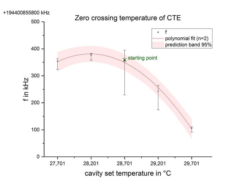
5.3 Zero-crossing Temperature Measurement
The zero-crossing temperature was measured at Menlo Systems and determined to be
at a set-temperature3 of 28.701 ◦C. To check this setting four measuring points around
this preset zero-crossing temperature were taken at 27.701 ◦C, 28.201 ◦C, 29.201 ◦C and
29.701 ◦C. The measurements took place over the course of three months, from February
to May 2021.
Setup
Again, the data was collected with a beating measurement between the ORS and the
ULN frequency comb (see fig. 5.1). The starting point of the measurement series was the
nominal zero-crossing point of 28.701 ◦C. The temperature of the cavity was then slowly
changed by half a degree to the next measuring point. A slow change of temperature
is necessary, so that the lock to the cavity is not lost. After changing the cavity’s
temperature, the ORS’s frequency takes roughly five days to settle and display a steady
linear drift of around 20 mHz/s. The frequency change due to thermal expansion of the
cavity is in the range of several hundred kHz. Due to the long settling time in-between
measurements the data points have to be corrected for linear drift, which is in the range
of several kHz per day.
Results
The measured data and the overall shape of the distribution of the data appear to suggest
that the zero-crossing temperature of the coefficient of thermal expansion is around
28.2 ◦C rather than the preset set point of 28.7 ◦C (see fig. 5.7). This result will have
to be checked by another measurement series in the future to verify the determined
zero-crossing temperature. At present, however, this is not possible as it requires a
time slot of at least three weeks with minimal traffic in the laboratory and no other
measurements running.
5.4 Uncertainty Budget
In order to provide an expanded uncertainty for the ORS’s frequency, which is traceable
to the BEV’s frequency standard, an uncertainty budget based on the principles of the
“Guide to the expression of uncertainty in measurement” (GUM, [Joi08]) was constructed.
In a first step one must define the measurand which is in this case the frequency of the
ORS measured with the ULN frequency comb generator. The measurement set-up has
three major components that will contribute to the uncertainty budget: the laser itself,
the reference frequency and the combined measuring system frequency comb and counter.
The estimate for the contributions from the frequency comb, which includes most of
the reference frequency’s uncertainty contribution, was obtained following the procedure
3
The displayed value by the built-in sensor will converge to this value.
38Sie können auch lesen