Setup and characterisation of a gas mixing unit for the dilution of CO 2 with N 2
←
→
Transkription von Seiteninhalten
Wenn Ihr Browser die Seite nicht korrekt rendert, bitte, lesen Sie den Inhalt der Seite unten
Setup and characterisation of a gas
mixing unit for the dilution of CO2
              with N2

           Bachelor thesis by

               Luana Rubino

              November 5, 2020

        University of Stuttgart

               Faculty 08

        5th Institute of Physics

     Examinar Prof. Dr. Tilman Pfau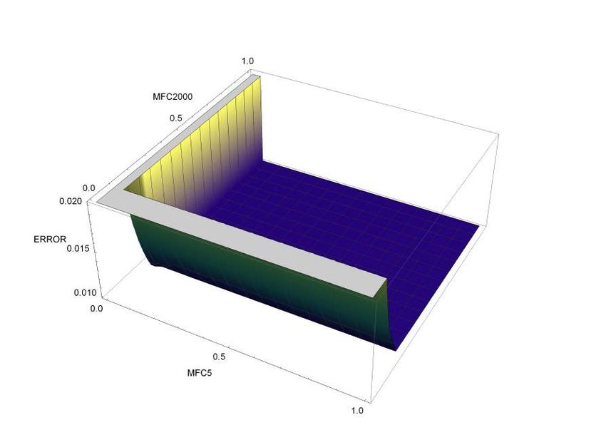
2
Erklärung

Hiermit erkläre ich, dass nach der Prüfungsordnung der Universität Stuttgart für den
Bachelorstudiengang Physik vom 31. Juli 2015 nach §27 Absatz 7 die Bachelorarbeit
die folgende Punkte versichert

  • dass die Arbeit selbständig verfasst wurde,

  • dass keine anderen als die angegebenen Quellen benutzt und alle wörtlich oder
    sinngemäß aus anderen Werken übernommenen Aussagen als solche gekennzeichnet
    sind,

  • dass die eingereichte Arbeit weder vollständig noch in wesentlichen Teilen Gegen-
    stand eines anderen Prüfungsverfahren gewesen ist, und

  • dass das elektronische Expemplar mit den anderen Exemplaren übereinstimmt

Luana Rubino
Stuttgart den 05. November 2020

                                         3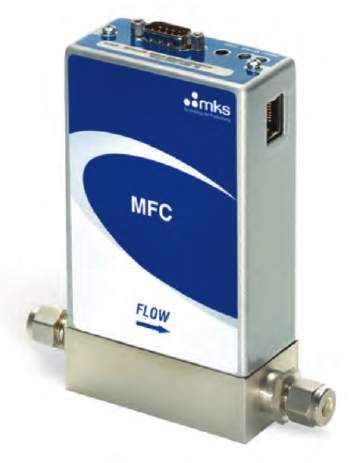
4
Deutsche Zusammenfassung

Ziel dieser Arbeit war es, ein Gasmischsystem für die Gase NO und N2 aufzubauen
und zu planen. Da die Struktur mit Rohren zusammengebaut ist, sollte hierfür der
Durchmesser bestimmt werden, was in Kapitel 2 mit der Berechnung der Knudsen-Zahl
Kn und der Reynolds-Zahl Re erfolgt.

Für eine laminare Strömung kann in diesem Aufbau ein Durchmesser von d = 4 mm
zugewiesen werden. Für einen konstanten Durchfluss werden Massendurchflussregler
(MFCs) verwendet, um unterschiedliche Mischungsverhältnisse zu erzeugen. Die Funk-
tionsweise wird in Abschnitt 3.1 betrachtet. Sie basiert auf der thermischen Massenbewe-
gung, die mit Hilfe der spezifische Wärmekapazität in einen Massedurchfluss umgerech-
net werden kann. Zur Messung der Konzentration nach den MFCs wird ein CO2 Sensor
verwendet, der die Infrarotabsorption der Moleküle misst was im Kapitel 3.4 näher er-
läutert wird. Für die Untersuchung des Systems, das für N2 und NO Gas ausgelegt ist,
werden Messungen mit CO2 und N2 Gas durchgeführt, da es einfacher zu handhaben ist
als NO Gas.

In Kapitel 4 Messungen und Auswertungen werden die MFCs und der CO2 Sensor un-
tersucht. Bei der Untersuchung des CO2 Sensors während der Aufzeichnung der Daten
wurde festgestellt, dass die lange Zeitverzögerung auf die Tatsache zurückzuführen ist,
dass es einige Zeit dauert, bis eine festgelegte Gleichgewichtskonzentration im CO2 Sen-
sor vorliegt, die nicht optimal ist, da die Mischverhältnisse nicht nach einer beliebigen
Zeit verändert werden konnten. Die MFCs wurden bei der Untersuchung der Kombi-
nationen auf konstante Konzentrationen berücksichtigt, was dazu geführt hat, dass für
2000 ppm und 4000 ppm CO2 in Bezug auf den Gesamtfluss Ftot beobachtet wurde. In
allen gemessenen Daten hat der CO2-Sensor einen sehr hohen Einfluss auf die Fehler-
balken, die fast ausschließlich aus dem Sensorfehler bestehen, was die Auswertung der
MFCs nicht vereinfacht.

Das mit Mathematica gelöste Skript in Anhang 2 bietet eine analytische Lösung für die
MFCs. Hier werden die Kombinationen von MFCs ohne Sensor betrachtet, hierzu werden
die Bilder in Abschnitt 4.3 gezeigt. Die Abbildungen zeigen deutlich den kleinsten
Fehler für die jeweiligen Kombinationen zweier MFCs für einen Gesamtfluss von Ftot =
1000 sccm und eine Verdünnung von D2 = 1/1000.

                                           5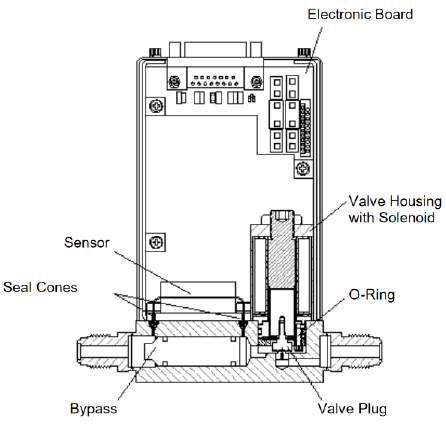
6
Contents

   1   Introduction . . . . . . . . . . . . . . . . . . . . . . . . . . .    .   .   .   .   .   .   .    9
   2   Theoretical Background . . . . . . . . . . . . . . . . . . . .        .   .   .   .   .   .   .   11
       2.1    Movements of gases . . . . . . . . . . . . . . . . . . .       .   .   .   .   .   .   .   11
       2.2    Ideal gas . . . . . . . . . . . . . . . . . . . . . . . . .    .   .   .   .   .   .   .   13
       2.3    Real gas . . . . . . . . . . . . . . . . . . . . . . . . .     .   .   .   .   .   .   .   14
       2.4    Thermal particles . . . . . . . . . . . . . . . . . . . .      .   .   .   .   .   .   .   14
       2.5    Non-dispersive infrared (NDIR) gas sensor . . . . . .          .   .   .   .   .   .   .   15
       2.6    Heat capacity C . . . . . . . . . . . . . . . . . . . . .      .   .   .   .   .   .   .   18
   3   Setup . . . . . . . . . . . . . . . . . . . . . . . . . . . . . . .   .   .   .   .   .   .   .   21
       3.1    Mass flow controllers (MFC) . . . . . . . . . . . . . .        .   .   .   .   .   .   .   21
       3.2    Gas pipe system . . . . . . . . . . . . . . . . . . . . .      .   .   .   .   .   .   .   23
       3.3    Valves . . . . . . . . . . . . . . . . . . . . . . . . . .     .   .   .   .   .   .   .   26
       3.4    CO2 sensor . . . . . . . . . . . . . . . . . . . . . . .       .   .   .   .   .   .   .   27
   4   Measurements and evaluation . . . . . . . . . . . . . . . . .         .   .   .   .   .   .   .   29
       4.1    Error values of the components . . . . . . . . . . . .         .   .   .   .   .   .   .   29
       4.2    Measurements . . . . . . . . . . . . . . . . . . . . . .       .   .   .   .   .   .   .   30
       4.3    Mathematical treatment of the dilution and total flow          .   .   .   .   .   .   .   34
   5   Conclusion and outlook . . . . . . . . . . . . . . . . . . . . .      .   .   .   .   .   .   .   39

1 CO2 sensor                                                                                             41

2 Choice of MFCs                                                                                         43

Bibliography                                                                                             45

                                            7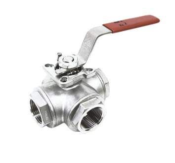
8
1 Introduction

Nitric oxide (NO) is a linear molecule found in many biological and chemical processes
[1]. Apart from various processes in the human body, NO can be synthesized from
the aminoacid L-arginine [2]. It is known that the concentration of NO of the exhaled
air gives information about the inflammatory status of the airway for asthma patients
[3]. For detailed information about the amount of the NO concentration in the exhaled
breath, breath gas analysis is necessary. This gas analysis can be done with an NO
sensor, for example with a optogalvanic sensor [1], which optically excites NO to a
Rydberg state [30] by collisions with ions and the background gas, which then measures
the resulting charges. The approximated detection limit of this sensor is at 5 ppb [1].

The gas mixing system built here is one part of a large project that deals with trace
gas. The gas mixing system is there to generate known mixing ratios between NO and
N2 which the NO sensor can then measure. The sensitivity of the NO sensor can be
improved by reducing the sample volume.

It is known that NO is toxic in high amounts which makes experimenting with it dan-
gerous. This is the reason why this thesis uses CO2 instead of NO for testing the gas
mixing unit with a known sample. Another advantage of this is that CO2 sensors are
cheaper than NO sensors. Since the only thing that differs in the setup is the type of
sensor needed, the setup for the characterization of the gas mixing unit stays the same.
Because an optogalvanic gas sensor measures the concentration of the trace gas (NO
or CO2), a constant mass flow is essential for achieving reliable results. This thesis is
an attempt to achieve a specific mixing ratio with constant mass flow by utilizing four
different mass flow controllers (MFC).

This thesis begins with a theoretical background where an overview of different gas
models is given. In this section, it is discussed why the mixed gases used in this thesis
can be approximated as ideal gases. The basic principle of a non-dispersive infrared
(NDIR) gas sensor and a MFC is discussed there, too.

After that the setup is described component by component. It begins with the MFCs,
their internal setup and technical information. The measurement technique is explained
in detail. A description of the gas pipe system built for this thesis follows. It is made
clear which components are needed to get laminar flow. Based on that the requirements
to the valves are given since they have to be NO resistant. In the last section the
principle of the used CO2 sensor is explained followed by its physical background.

In the measurements and evaluation chapter an interpretation of the measured data is
given. This contains a brief characterisation of the CO2 sensor, the flow changing be-
havior of different MFCs combinations and the dependency on the concentration change
for the forward and backwards direction of the CO2 sensor.

                                           9
10
2 Theoretical Background

This chapter gives an overview about the movements of gases, as well as the laws of gases.
Also important is the technology how a non-dispersive infrared gas sensor measures and
finally the heat capacity is considered.

The following explanation is mostly based on [4].

2.1 Movements of gases

A closer look into gas dynamics shows that there are two significant flow types: molecular
and viscose flow. These types are observed in a pipe with a volume V , the cross-section
A and length h.

The molecular flow dominates at low pressure where the mean free path is much larger
compared to the pipe diameter. The only interaction the molecules have is with the
pipe. In case of the viscose flow type, the pressure is much higher. This means the mean
free path is much smaller and the probability of molecules hitting each other is much
higher.

To distinguish the molecular flow and the viscose flow the Knudsen number Kn is
introduced. The Knudsen flow describes the interaction with the pipe and molecules
more or less equally weighted. Therefore, the Knudsen number can be calculated to
determine whether the flow is molecular or viscose.

The Knudsen number Kn is defined as:
                                                λ
                                        Kn ≡                                         (2.1)
                                                l
In equation (2.1) λ is the mean free path of the molecules in meters and l is a repre-
sentative physical length scale in meters. For example for a pipe, l it is the diameter.
A number between Kn = 0.5 to Kn = 0.01 defines a Knudsen flow. If Kn > 0.5 it
describes molecular flow, for Kn < 0.01 it is viscose flow.

As an overview, table 2.1 gives Knudsen numbers for different pipe diameters. The
mean free path for CO2 is λCO2 = 45 nm [17] at temperature T = 20 °C and a pressure
of p1 = 1 bar. For p2 = 10 mbar and T = 20 °C the mean free path is λCO2 = 4.5 µm
[17].

                                           11
Table 2.1: Knudsen numbers of CO2 for different pipe diameters
l [mm] 2 3 4 5 6 7 8 9 10
−5
Kn1 [10 ] 2.25 1.5 1.125 0.9 0.75 0.64 0.5625 0.50 0.45
Kn2 [10−5 ] 225 150 112.5 90 75 64.3 56.25 50 45
Another important property is the characterisation of gases with a viscose flow, where
the speed through the pipe is important. Considering the speed, there are two signifi-
cant gas flow models: the laminar flow and the turbulent flow. In figure 2.1c) turbulent
flow is visualised. As the name indicates it is a turbulent flow what means that here
vortices arise. This happens when the center of the pipe and the edges have a huge
difference in velocity. In case of big velocity differences it happens that the middle and
the edges of the pipe generate friction forces which lead to turbulent flow. For laminar
flow the velocity difference is much less which leads to no turbulent flow. Laminar flow
is often described as layers with different velocities like the arrows in figure 2.1b). Here
the velocity slows down on the edges but is parallel to the other layers.
a) b) c)
v v
Figure 2.1: This figure describes three different flow types. a) the gas flow enters the
pipe and collides with the inner wall of the pipe which is called molecular
or ballistic flow. b) shows a laminar flow whereby the velocity vectors are
pointing in the same direction, no vertices arise because friction forces to
each other are very low. c) shows turbulent behavior which happens due
to high velocity of the gas which means the velocity difference between the
middle of the pipe and the edges is high. At this picture the length of the
vector is proportional to the speed. The type of flow does not only depend
on the speed, which can be read from the Reynolds number, the diameter,
the dynamic viscosity and the density are also relevant. After [4].
The Reynolds number Re indicates whether the flow is laminar or turbulent. The
Reynolds number is defined as
ρ
Re ≡ · v · l. (2.2)
µ
In equation (2.2) ρ is the density in [kgm−3 ], µ the dynamic viscosity in [kg m−1 s−1 ], v
the flow velocity in [m s−1 ] and l a representative physical length scale in [m]. A Reynolds
12number higher than 4000 defines a turbulent flow and a Reynolds number smaller 2300
defines a laminar flow. Inside of this range it is called Reynolds flow.
The velocity v can be calculated by the time derivative of the Volume V divided by the
cross-section area A of the pipe. Now the Reynolds number can be described like in
equation (2.3) where h is the length of the pipe. It depends on the diameter l and the
time t the gas particles take to pass through the pipe.
V̇ h ρhl
v= = ⇒ Re = (2.3)
A t µt
As an example CO2 has the density ρ = 1.815 kg/m3 and the dynamic viscosity µ =
14.69 · 10−6 kg m−1 s−1 at pressure p = 1 bar and temperature T = 20 °C [18]. A few
Reynolds numbers of CO2 are shown in table 2.2.
Table 2.2: Reynolds numbers of CO2 for different pipe diameters l and different flow
times t at the length of h = 4 m.
v [m s−1 ] ReCO2 l = 3 mm 4 mm 5 mm
1.33 t = 3s 4942 6589 8236
1 4s 3706 4942 6177
0.8 5s 2965 3953 4942
0.66 6s 2471 3294 4118
0.57 7s 2118 2824 3530
0.5 8s 1853 2471 3088
0.44 9s 1647 2196 2745
2.2 Ideal gas
An ideal gas describes an idealized representation of the gas, whereby the gas molecules
are viewed as point particles which move statistically. After and before the collision,
they move evenly and independently. These point particles can elastically collide with
each other and thus transfer energy. Because these are seen as point particles, the only
energy they exchange is the kinetic energy. Forces acting on one another, such as the
Van-der-Walls force, are not taken into account here. The basic equation for gases which
is valid for moving points as particles is known as the ideal gas law (2.4).
pV = N kB T (2.4)
In equation (2.4), p describes the pressure in [bar], V the volume in [m3 ], N the number of
molecules, kB = 1.3806·10−23 m2 kg/s2 K the Boltzmann constant and T the temperature
in [K]. The ideal gas law is a combination of Boyle-Mariotte’s law, Gay-Lussac’s law, and
Avogadro’s law. Boyle-Mariotte’s law means that at a given temperature T the volume
13is reversely proportional to the pressure p as defined in equation (2.5). Gay-Lussac’s
law describes a proportionality between the volume and the temperature T as defined
in equation (2.6) while the pressure is constant. The last essential law is described by
Avogadro, saying that the volume V is proportional to the number of particles n for
constant pressure p as well as for constant temperature T (2.7).
1
V ∝ : Boyler-Mariotte’s law (2.5)
p
V ∝T : Gay-Lussac’s law (2.6)
V ∝n : Avogadro’s law (2.7)
2.3 Real gas
The following explanation is mostly based on [13].
The ideal gas law is valid for moving points which do only interact fully elastic. Real
gases instead have extended particles where different forces between the molecules can
arise. Attraction and repulsive forces are present, in the following the attraction Van-
der-Waals force is considered.
A closer look into the Van-der-Waals force, which describes a very weak force where the
interaction between dipoles is considered. The Van-der-Waals force gives a volume and
pressure adjustment of the ideal gas law. For molecules, the real volume
is (V− nb)
2
n
with b as the molecules own volume, while the real pressure becomes p + a V
with
a as the aspect ratio factor. Equation (2.8) shows the real gas law, with n as amount of
substance and a, b as Van-der-Waals constants.
2 !
n
p+a · (V − nb) = N kB T (2.8)
V
2.4 Thermal particles
The following explanation is mostly based on [6] and [7].
Particle velocity
In reality, there are inelastic collisions between particles which lead to a velocity dis-
tribution described by the Maxwell-Boltzmann-distribution f (v) as defined in equation
14(2.9) with m as mass in [kg] of the particle.
−mv 2
3
m
2
2
f (v) = 4πv e 2kB T (2.9)
2πkB T
As for every probability distribution there is a most probable value of the velocity as
defined in equation (2.10) √
and an average velocity as defined in equation (2.11). These
values are proportional to T , for larger temperatures the probability distribution f (v)
gets wider whereby the average speed shifts to a higher speed what figure 2.2 shows.
s
2kB T
v̂ = (2.10)
m
s
Z ∞
8kB T
v= vf (v)dv = (2.11)
0 πm
1.6
1.4 T1
1.2 T2 > T1
Probability f(v)
1
0.8 T2
0.6
0.4
0.2
0
0 10 20 30 40 50 60 70
Velocity v
Figure 2.2: The probability f (v) is plotted against the velocity v for two different tem-
peratures T1 and T2 . At higher temperatures the most probable value v̂ is
less higher and shifted to the right and the velocity distribution gets wider on
the velocity axes, because the area below the graph needs to be normalized.
2.5 Non-dispersive infrared (NDIR) gas sensor
Technique
This technique is used for gas sensing. It is based on infrared spectroscopy, by which the
molecules absorb energy at resonant frequencies. Every molecule has different vibrational
15frequencies, with this knowledge the molecules can be distinguished from each other.
The frequency for which it is resonant depends on the vibrational movement of the
molecules. In figure 2.3 the different possibilities of a CO2 molecule to vibrate are
shown. Vibrational movements can be described with the Lorentz model where the atoms
act like if they were connected with springs. Every movement has its own resonance
frequency which is shown in figure 2.4. The movements are described in figure 2.3: a)
the asymmetric stretch where the carbon and oxygen atoms are moving in one plane but
in different directions is shown, b) the symmetric stretch where only the oxygen atoms
are moving is shown and c) the two degenerated bends where the molecule is moving is
shown.
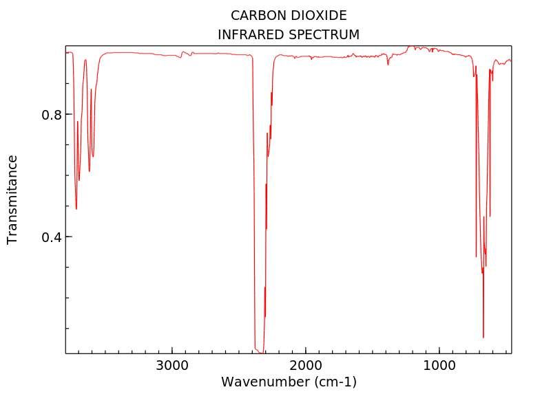
The infrared spectrum in figure 2.4 shows which peaks are assigned to which movement.
The central dip belongs to the asymmetric movement which means at this wavenumber
the transmittance is very high [28]. The degenerated bends are absorbing infrared light
at a much lower wavenumber compared to the asymmetric movement which is described
by the right dip in figure 2.4.
a) O c O
b) O c O
c) O c O
Figure 2.3: The fundamental vibrations of a CO2 molecule are shown here. From top to
bottom: the asymmetric stretch, the symmetric stretch and the degenerated
bends.
16Figure 2.4: Shows the infrared transmission dips for a CO2 molecule. The two larger
dips are approximately at 2325 cm−1 = 4.3 µm and at 654 cm−1 = 15.3 µm
which are caused by the asymmetric stretch and the degenerated bands [28].
Taken from [26].
Construction
The schematic of the sensor is shown in figure 2.5 as a basic sketch. The gas can enter the
chamber at one point and can escape at another point. The infrared source illuminates
the chamber up to the other end, where an optical filter and a detector are placed. If
the chamber is filled with gas, the infrared source shines through it. The gas absorbs
different frequencies, depending on the molecules of the gas. The optical filter is for
suppressing the background noises.
The disadvantage of this system is the pressure dependence which influences the absorp-
tion measurements. The advantages are that the sensor only has an infrared source and
a detector. This advantages results in a small sensor.
17Figure 2.5: Schematic of the CO2 sensor where the gas enters at one part and escapes
at the other one. With an infrared source which illuminates through the
chamber it can detect the molecules by absorption. The optical filter helps
suppressing the background. After [9].
With the Beer-Lambert law [29], which compares the intensity I0 from the incoming
infrared source and the intensity I from the detector, the equation (2.12) gives the
concentration c of the CO2 gas which depends on the background pressure. I0 can be
determined from the calibration of the sensor.
I = I0 e−kcl (2.12)
In equation (2.12) k is the absorption coefficient, and l is the optical absorption path.
The concentration can be calculated with equation (2.13).
I0 1
c = ln · (2.13)
I kl
2.6 Heat capacity C
The heat capacity C can be derived from the first law of thermodynamics. It represents
a material property which depends on the change of the heat Q and temperature T .
First law of thermodynamics
The first law of thermodynamics (2.14) describes the energy change between the internal
energy dU , the heat energy dQ and the work dW .
dU = dQ − dW (2.14)
18The internal energy dU is composed of the heat energy dQ and the work dW . Consid-
ering a gas in a volume V the internal energy is getting bigger by heating up the gas.
The reason is that the particles gain kinetic energy Ekin , this energy is divided by three
different possibilities to gain energy. These possibilities are defined by the degrees of
freedom f which are consisting of a translation, a rotation and a vibration part. As
shown in table 2.3, there are differences between monatomic and N −atomic molecules.
For one atom it is only possible to move in the three-dimensional space, it can’t rotate or
vibrate. For N −atomic molecules, vibrational and rotational degrees of freedom exist.
For example, a linear molecule (figure 2.3) like CO2 has nine degrees of freedom, two
rotational and four vibrational degrees of freedom.
Table 2.3: Degrees of freedom f for a atom and a N -atomic molecule
fi atom N -atomic
linear non-linear
translation ft 3 3 3
rotation fr 0 2 3
vibration fv 0 3N − 5 3N − 6
total ftot 3 3N 3N
Derivation
Knowing that changing the heat energy the temperature also changes i.e. dQ ∼ dT , the
proportionality factor C is called heat capacity (2.15).
dQ
C= (2.15)
dT
The heat capacity is a material property, hence it depends on the mass m. The mass
dependency is shown in equation (2.16) which is called specific heat capacity.
C 1 dQ
c= = (2.16)
m m dT
A distinction can be made between the specific heat capacity for constant pressure cp
and constant volume cV .
1920
3 Setup

The setup consists of different parts, four mass flow controllers (MFC), a gas pipe system,
valves and a CO2 sensor, which depend on each other. The main part is the gas pipe
system, where the gas first flows through the pipes to the MFCs to be mixed and
then from the MFCs to the CO2 sensor where the gas is then transported away by
the gas extraction. The pipes and pipe connections have been selected to be suitable
for laminar flow by calculating the Reynolds number and the Knudsen number. One
requirement for this setup is a constant mass flow which can be generated with so-called
mass flow controllers from MKS. This requirement comes from the fact that the setup
is designed for an NO sensor which requires a constant mass flow and should measure
low concentrations. Another requirement is that a dilution factor of 10000 should be
achievable, the range in which these MFCs should be able to mix is the ppb range,
clarified in percentage it is 0.000 000 1 %.

This setup is constructed for the gases NO and N2 which means that the different parts
have to be leak-proof and resistant otherwise NO reacts directly with O2 to NO2 which
is very toxic. The gas paths were chosen so that NO is not able to get into the N2
gas container, as these components are not designed for NO where only N2 should pass.
Since the gases NO and N2 should not be mixed before the MFCs, valves are used to
prevent this. Therefore, only the gases N2 and CO2 were used for testing. For this setup,
a CO2 sensor is used to investigate the MFCs.

3.1 Mass flow controllers (MFC)

The mass flow is controlled by the MFCs. They are an important part in this setup to
produce a continuous controlled mass flow. To get as much variety as possible in mass
flow the flows should be adjustable. As an overview, table 3.1 shows the available MFCs
with the given flow ranges. These four MFCs were chosen so that the respective flow
areas can overlap and thus the system can go from 0.1 sccm to 52 105 sccm.

Figure 3.1 shows a MFC, it has one inlet and one outlet for the gas, and at the top
part a D-Sub plug and an Ethernet connection. Two LEDs, also at the top, indicate the
status of the MFC.

                                            21
Figure 3.1: Mass flow controller from MKS, taken from [14]
Table 3.1: Flow ranges of the MFCs
MFCs Flow ranges
MFC1 1000 to 50000 sccm
MFC2 40 to 2000 sccm
MFC3 2 to 100 sccm
MFC4 0.1 to 5 sccm
A closer look at the inside of a MFC in figure 3.2 shows how it is built. First of all, the
flow path of the gas goes through the entry and splits into two parallel ways. One way is
through the bypass which is adjustable and the other is through the sensor pipe. After
that, both ways are recombined and lead through the control valve to the outlet.
22Figure 3.2: Assembly of the MFCs from MKS. It works by measuring the thermal mass
movement which than can be concerted with the specific heat capacity cp to
obtain the mass flow. The gas flows from the left to the right side. Taken
from [15].
The measurement technique, which is formulated in [15], is based on measuring the
thermal mass movement with heat transfer between temperature sensing elements, which
than can be converted with the specific heat capacity cp to obtain the mass flow. By
amplifying, digitalising and linearizing the signal it is sent to the control section where
it is transform in a 0 − 5 V analog signal which can be read out.
3.2 Gas pipe system
The basic idea is to build a setup for N2, NO and N2/NO 100 ppm or even lower (10 ppm)
gas, with four MFCs. Looking at figure 3.3, the basic idea of this setup is shown. Two
different gas inlets are used here, because the NO should not be able to get into the N2
gas container, as these components are not designed for NO, a leak can be dangerous for
the experimenters because its react directly with O2 into the red-brown nitrogen dioxide
NO2. It is to be recognized that the NO gas course only goes to the three lower MFCs
because the amount of required total flow is covered with the lower ones.
23Legend:
MFC1 Three way ball valves
N2 One way ball valves
Free way cross
MFC1: 50000 sccm
MFC2 MFC2: 2000 sccm
MFC3: 100 sccm
MFC4: 5 sccm
MFC3
CO2 sensor
N2/NO
MFC4
Gas extraction
NO
Figure 3.3: It is illustrated the gas pipe setup with MFCs, CO2 sensor, valves and free
way crosses with two inlets. The gases can flow through the MFCs to the CO2
sensor which measures the concentration and the gas extraction transports
the gas out of the system.
Pipes
As calculated in table 2.1 and 2.2, it is possible to choose different diameters for laminar
flow in the pipes. In this experiment, an outer diameter of d = 6 mm and an inner
diameter of d = 4 mm is used. An important requirement about these pipes is that they
are seamlessly made of stainless steel which makes them more stable for high pressures.
24Figure 3.4: Shown are here stainless steel pipes which are seamless [21]
Pipe connections
Cutting rings are very important components in this setup, they seal the screw cap
between every pipe to MFC connections and also pipe to valve connections. Two different
cutting rings were used here. The first one is from Landefeld, shown in figure 3.5 and the
second one is from Swagelok, illustrated in figure 3.6. They are slightly different from
each other. The rings from Landefeld are one-piece, while the ones from Swagelok are in
two parts. They are sitting in between the pipe and the union nut, by tighten the union
nut up, the cutting rings are cutting themselves in the pipe which seals everything.
Figure 3.5: Shown here is a cutting ring
from Landefeld [22].
Figure 3.6: Shown here is a cutting ring
from Swagelok with union
nut[24].
253.3 Valves
Three way ball valve
The three way ball valve in figure 3.7 is an NO resistant valve sealed with PTFE. In
the center of the valve a ball is located, which gives the direction of the flow. The ball
is not completely filled, the part which is missing gives the opening of the valve. The
direction of the flow depends on the borehole, this three way ball valve have a L-drilling
which is important because NO shouldn’t get a chance to get to the N2 container.
With the handle at the top, the ball can be moved in the desired direction. A three
way ball valve is used in figure 3.3 wherever the different gases can’t collide with each
other.
Figure 3.7: Shown is here a three way ball valve [16]
One way ball valve
The one way ball valve is similar to the three way ball valve, the difference is that the
one way ball valve has only the setting opened or closed. The entrance is regulated with
a ball like the three way ball valve.
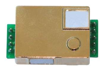
263.4 CO2 sensor
The CO2-sensor (figure 3.8) is a non-dispersive infrared sensor from the brand Zhengzhou
Winsen Electronics Technology Co., Ltd, Model: MH-Z19B. The pin assignment is shown
in figure 3.8 b), a closer look on that shows there are two ways to read the data: quasi
analog (PWM) and digital (UART). The required pins for the UART-measurement
are Tx and Rx which are transmitter and receiver.
The two white areas in figure 3.8 a) are the inlet and the outlet where the gas can enter
and leave the sensor.
The sensor can be zero calibrated by connecting the HD pin with the low level V0 pin
at least for seven seconds.
(a) CO2 sensor (b) Pin assignment
Figure 3.8: A CO2 sensor from the brand Zhengzhou Winsen Electronics Technology Co.,
Ltd with the model number MH-Z19B[23]
Measuring with UART
The measurements by using UART were recorded with an Arduino Nano by using the
script from [25] which can be found in appendix 1.
The measuring process was as follows: The first thing to do is to calibrate the sensor,
which is done by connecting pins HD and V0 and these for seven seconds when the sensor
is connected, which then has to be left for about twenty minutes. After the calibration,
the sensor is connected to the Arduino to establish a connection. For the required gas
flow, the gas valves are set in the required position and the gas is let through. So that
the sensor can measure the concentration, the MFCs are set to the desired setting, now
the sensor should be able to measure something. The script from Chapter appendix 1
is executed so that the sensor measures the concentration of CO2 in [ppm].
2728
4 Measurements and evaluation

The aim of this chapter is to achieve the best combination of MFCs with minimum error.
Starting with basic equations in chapter 4.3 and continuing with the error values of the
components 4.1, the total flow and the dilution of the MFCs can be calculated. Chapter
4.2 shows the behavior of the MFCs and the CO2 sensor and finally in chapter 4.3 the
choice of the right combination for the MFCs will be discussed.

4.1 Error values of the components

The main error value comes from the CO2 sensor which is much higher than the one
from the MFCs. In the following, the error values of the Sensor and the MFCs will be
described.

CO2 sensor

The accuracy ∆S of the CO2 sensor is formulated in equation (4.1) and can be found in
the data sheet [23].

                       ∆S = ± (50ppm + 5% of reading value)                        (4.1)

Section 4.2 shows the accuracy for the values which mostly originate from the sensor.

For the difference D (4.2) between the values of the CO2 sensor and MFCs, the error
can be calculated with equation (4.3). The difference D consists of the CO2 sensor value
and the values from the MFCs, which are given in [sccm], for the two gases which is
multiplied with 106 due to the unit from the CO2 sensor, it is in [ppm].
                                                CO2 6
                                 D = Sensor −       10                             (4.2)
                                                 N2
                               ∂D         ∂D        ∂D
                       ∆D =        ∆CO2 +     ∆N2 +    ∆S                          (4.3)
                              ∂CO2        ∂N2       ∂S

MFCs

The MFCs have the accuracy [14]

  • ± 1% of set point for 20 to 100% Full Scale and

                                          29
• ± 0.2% of Full Scale for 2 to 20% Full Scale
With the equation for the MFCs (4.4), which gives the mixing ratio in [ppm], is used
for the evaluation, the error can be calculated with equation (4.5).
CO2 6
M= 10 (4.4)
N2
!
1 CO2
∆M = ∆CO2 + ∆N2 106 (4.5)
N2 N22
The MFCs have some restrictions as their control range is 2% to 100% of full scale for
N2, for any other gases this value can be slightly different, which depends from the gas
type. This difference results from the specific heat capacity cp which is gas dependent.
4.2 Measurements
In the following the investigation of the CO2 sensor and the MFCs is given. Questions
like "Does the flow change by using different MFCs?" or "Does the CO2 sensor have some
time delay?" will be clarified. The error bars listed here are calculated as described in
chapter 4.1.
The measuring process is as follows: First of all, the CO2 sensor is connected to the
Arduino, which evaluates the data. Additionally the CO2 sensor needs a separate power
connection. Then by programming the Arduino with appendix 1, the sensor can be read
out. The time and the concentration were read out for the following evaluations. The
readout of the MFCs which gives the mass flow for the gases N2 and CO2 can be accessed
via the website.
Time delay ∆t of the CO2 sensor
When measuring the time delay ∆t, the CO2 concentration and the time t are measured.
By changing the CO2 concentration the CO2 sensor needs a certain time to get to its
final value. For three concentration changes, figure 4.1 shows how much time the sensor
needs to reach the final value. The time differences ∆ti in figure 4.1 are ∆t2→1 = 407 s,
∆t4→3 = 448 s and ∆t6→5 = 481 s. These values are pretty similar to each other which
suggests that the time delay is constant. The long time delay comes from the fact that
it takes time to have a set equilibrium concentration in the chamber. A disadvantage
about this is that the concentration change can’t be done fast.
305000 CO2−sensor
t1 = 1128 s
4551 ppm
4500 3530 ppm
t2 = 1535 s
2460 ppm
4000 t3 = 1691 s 1351 ppm
CO2 [PPM]
3500
t4 = 2139 s
3000 t5 = 2221 s
2500
2000
t6 = 2702 s
1500
1000
1000 1500 2000 2500
Time t [s]
Figure 4.1: Demonstration of the time delay of the CO2 sensor for different concentration
changes plotted against time t. The time delays are: ∆t2→1 = 407 s, ∆t4→3 =
448 s and ∆t6→5 = 481 s.
Investigation of different MFC combinations for concentrations of 4000 ppm and
2000 ppm
For this part, the concentration of the MFCs and the sensor were read out and the
difference D was calculated from these values and plotted against the total flow ftot .
The difference D describes the difference between the value of the MFCs and the value
of the CO2 sensor this is done because the calibration of the CO2 sensor is not accurate
enough which makes a different between the sensor and the MFCs.
This measurement was done for different combinations of two MFCs, MFC1 = 50 000 sccm
and MFC3 = 100 sccm were combined and MFC2 = 2000 sccm and MFC4 = 5 sccm
were used together, with concentrations of 4000 ppm and 2000 ppm.
In figure 4.2 it is shown how much the combination of the MFCs affects the difference
D for a concentration of 4000 parts per million (ppm) CO2. The combination of the
MFCs is shown in the legend with the associated mass flow rate, N2 to CO2. Besides,
sccm defines a unit which is called standard cubic centimeter per minute (cm3 /min).
No trend can be observed in the images 4.2 and 4.3 which means that the flow is not
changing for different MFC combinations. It should be noted, however, that the error
31bars in the figures are very large, which may result in a different looking figure when
using a better sensor with lower errors.
4000ppm
1150
1100
1050
1000
950
D [ppm]
900
850
800 1000sccm to 4sccm
500sccm to 2sccm
750 10000sccm to 40sccm
700 5000sccm to 20sccm
2500sccm to 10sccm
650
0 1 2 3 4 5 6 7 8 9 10 11
3
Ftot [10 sccm]
Figure 4.2: Difference D against the total flow ftot for a concentration of 4000 ppm
CO2. The concentration of the MFCs and the sensor were read out and the
difference was calculated from these values and was plotted against the total
flow. The different combinations of MFCs are shown in the legend of the
figure whereby the flow rate is represented as NO to CO2.
322000 ppm
700
600
D [ppm]
500
2000sccm to 4sccm
400 1000sccm to 2sccm
500sccm to 1sccm
20000sccm to 40sccm
300 10000sccm to 20sccm
5000sccm to 10sccm
2500sccm to 5sccm
200
0 2 4 6 8 10 12 14 16 18 20 22
Ftot [103 sccm]
Figure 4.3: Difference D to the total flow ftot for a concentration of 2000 ppm CO2. The
concentration of the MFCs and the sensor were read out and the difference
was calculated from these values and was plotted against the total flow. The
different combinations of MFCs are shown in the legend of the figure whereby
the flow rate is represented as NO to CO2.
Dependence of the concentration on the ramp direction
At this section, the concentration of the MFCs and the CO2 sensor were read out and
the difference D was calculated from the values and was plotted against the total flow
Ftot . This was done for concentrations of 4000 ppm, 3000 ppm, 2000 ppm, 1000 ppm and
500 ppm of CO2 to N2. For a constant flow of N2 = 1000 sccm, CO2 was changed so
that the concentration as shown in the figure 4.4 was reached. The time it took until
the concentration leveled off can be read off from section 4.2, this time was necessary to
wait.
Figure 4.4 shows the results. The chronological order of this measurements is the fol-
lowing: first red dots from 4000 sccm down to 500 sccm and second blue dots back again
from 1000 sccm to 4000 sccm. Figure 4.4 shows that comparing both functions there
are significant differences in the slope and the axis intercept of the fit function can be
recognized, but due to the large error bars it looks as if this was due to the measurement
error of the sensor.
33900
down
800 up
f(Ftot)
h(Ftot)
700
600
D [ppm]
500
400
300
200
100
0 1000 2000 3000 4000 5000
Ftot [sccm]
Figure 4.4: Ramping the concentration from low total flow to high total flow (blue)
and vice versa (red). The difference between the MFC and the sensor was
calculated and shown here. The red dots are going from a flow of 4000 sccm
down to 500 sccm and the blue dots back again from 1000 sccm to 4000 sccm,
for concentrations of 4000 ppm, 3000 ppm, 2000 ppm, 1000 ppm and 500 ppm.
The fit functions are: f (Ftot ) = 0.123 403 ppm/sccm · Ftot + 169.801 ppm and
h(Ftot ) = 0.155 424 ppm/sccm · Ftot + 248.988 ppm.
4.3 Mathematical treatment of the dilution and total flow
At this point in the evaluation, a mathematical consideration is made which estimates
an error and minimizes it. The CO2 sensor is not taken into account, because the
minimization of errors of the MFCs are simulated.
In this there are few important equations like the total flow Ftot (4.6) and the dilutions
Di (4.7), (4.8), (4.9). The dilution describes a ratio, e.g. D2 has considered a ratio
between flow of NO to total flow Ftot . xi can assume values from 0.02 to 1.
The total flow Ftot is defined as the sum over all MFCs with the maximum flow range
(table 3.1) multiplied with xi which gives the percentage of the MFCs divided by 100.
Ftot = 50000 · x1 + 2000 · x2 + 100 · x3 + 5 · x4 (4.6)
2000 · x2 + 100 · x3 + 5 · x4
D1 = (4.7)
Ftot
34100 · x3 + 5 · x4
D2 = (4.8)
Ftot
5 · x4
D3 = (4.9)
Ftot
MFC setting with minimal error
When looking at the MFCs, they have the following error, which depends on the set
flow [14]
• ± 1% of set point for 20 to 100% Full Scale
• ± 0.2% of Full Scale for 2 to 20% Full Scale
To obtain a minimum error for different combinations of MFCs, this can be calculated
analytically. With using the equations for total flow (4.6), the dilutions (4.7), (4.8) and
(4.9) and the error functions which can be generated from the data given from the upper
part, a linear system of equations can be formed. The linear system of equations does not
provide an unambiguous solution because it is under-determined with two independent
equations, with two parameters Ftot ans D and three unknowns xi . The result is a bevy
of solutions, which can be infinitely many or none exist.
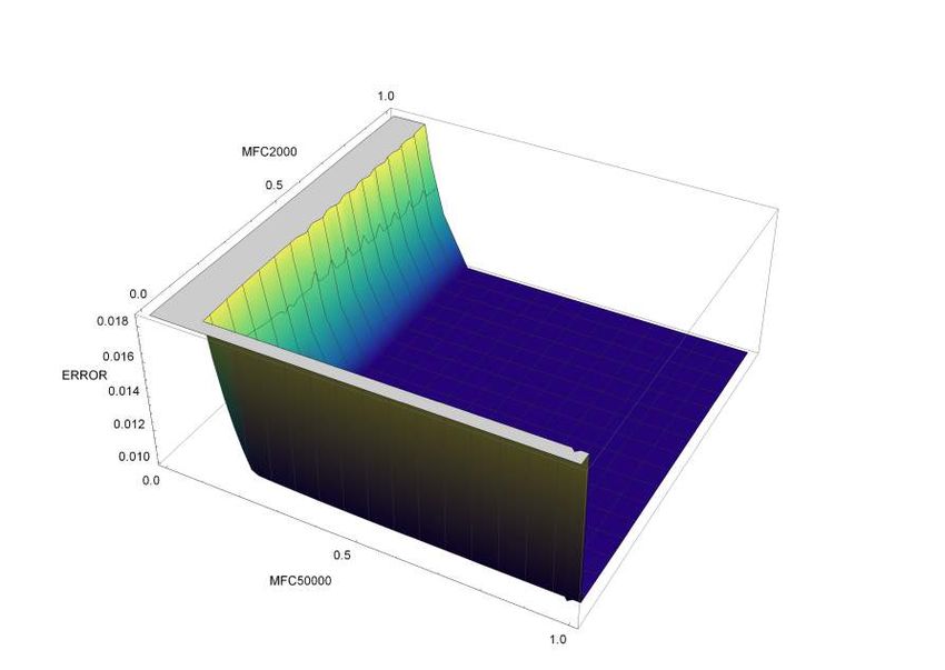
By using Wolfram Mathematica the script in appendix 2 was solved. The figures 4.5, 4.6
and 4.7 were created with this script. The figures show different combinations of MFCs
with a total flow of Ftot = 1000 sccm and a dilution of D2 = 1/1000. The dark violet
spots indicate a small error ranging up to yellow spots as the larger error range.
Figure 4.5 shows perfectly that smaller errors are obtained by choosing larger MFC in
the upper range, than the smaller ones in this range, which is also illustrated in figures
4.6 and 4.7. For the setup it means to rather choose a combination where the bigger
one is more open compare to the other one to have a larger full scale which minimize
the total error.
These pictures only shows one way to combine the MFCs for a total flow of ftot = 1000 sccm.
This script can go through any number of options by changing the total flow ftot and
the dilutions Di .
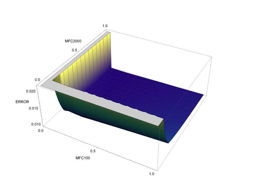
35Figure 4.5: The combination here is with the MFC2 = 2000 sccm and the MFC3 =
100 sccm, for this the script in Chapter 2 was carried out by Mathematica
for a total flow of ftot = 1000 sccm and the dilution of D2 = 1/1000 assumed.
The two MFCs are shown in the percentage range of 0% to 100% for 0% as
closed and 100% as completely opened and the associated error ERROR in
sccm, which is shown as a height map.
36Figure 4.6: The combination here is with the MFC2 = 2000 sccm and the MFC4 =
5 sccm, for this the script in Chapter 2 was carried out by Mathematica for
a total flow of ftot = 1000 sccm and the dilution of D2 = 1/1000 assumed.
The two MFCs are shown in the percentage range of 0% to 100& for 0% as
closed and 100% as completely opened and the associated error ERROR in
sccm, which is shown as a height map.
37Figure 4.7: The combination here is with the MFC2 = 2000 sccm and the MFC1 =
50 000 sccm, for this the script in Chapter 2 was carried out by Mathematica
for a total flow of ftot = 1000 sccm and the dilution of D2 = 1/1000 assumed.
The two MFCs are shown in the percentage range of 0% to 100% for 0% as
closed and 100% as completely opened and the associated error ERROR in
sccm, which is shown as a height map.
385 Conclusion and outlook
The aim of this work was to set up and plan a gas mixing system for the gases NO
and N2. The system was checked with CO2 gas which is less toxic and less expensive to
NO, and which was measured with a CO2 sensor. Since the structure is assembled with
pipes, the diameter d should be determined for these, which is done in chapter 2 with
the calculation of the Knudsen number Kn and the Reynolds number Re.
For a laminar flow, a diameter of d = 4 mm can be assigned in this setup. For a constant
flow, mass flow controllers (MFCs) are used to create different mixing ratios. The mode
of operation is considered in section 3.1, it is based on measuring the thermal mass
movement which than can be concerted with the specific heat capacity cp to obtain
the mass flow. To measure the concentration after the MFCs, a CO2 sensor is used,
which measures infrared absorption of the molecules and it is explained in more detail
in chapter 3.4. For the investigation of the system, which is designed for N2 and NO
gas, measurements are made with CO2 and N2 gas because it is easier to handle than
NO gas.
In chapter 4 Measurements and evaluations, the MFCs and the CO2 sensor are exam-
ined. During the examination of the CO2 sensor while recording the data, it was noticed
that the long time delay ∆t comes from the fact that it takes time to have a set equi-
librium concentration in the chamber which is not optimal since the recordings cannot
be changed after any time. The MFCs were taken into account when examining the
combinations for constant concentrations, which has resulted in the fact to be observed
for 2000 ppm and 4000 ppm of CO2 in relation to the total flow Ftot . In all measured
data, the CO2 sensor has a very high influence on the error bars, which consist almost
entirely of the sensors error, which does not simplify the evaluation of the MFCs.
The script in appendix 2, which was solved with Mathematica, offers a solution for the
MFCs, here, the combinations of MFCs are considered without the sensor, the images in
section 4.3 are shown for this. The figures clearly show the smallest error for every two
combined MFCs for a total flow of ftot = 1000 sccm and a dilution of D2 = 1/1000.
The next task to work on is to use this gas mixing system for the optogalvanic sensor,
the CO2 sensor is removed.
At the moment there are problems to bring the parameters under control, like the
pressure fluctuations in the measuring system, which makes the investigations unreliable.
The first step is to tested it with pure N2 to look if the pressure is stable. If the
measurements are accordingly to what the expectation is the setup is used for NO and
the mixing ratios are set.
3940
1 CO2 sensor

In the following, the script from [25] was presented in a brief version.

    # include < S oftwareS erial .h >

    // Port 2 ( RX ) and Port 3 ( TX )

    Softw areSeria l co2Serial (2 , 3); // define MH - Z19 RX TX

    void setup () {

         Serial . begin (9600);
         co2Serial . begin (9600);

    }

    // Reading out the sensor values ppm and temperature

    void loop () {

         int ppm , temperature = 0;
         readSensor (& ppm , & temperature );

    //     Serial . print (" PPM : ");
         Serial . print ( ppm );
         Serial . print (" ");
         Serial . println ( temperature );

         delay (1000);
    }

    void readSensor ( int * ppm , int * temperature ){

         byte cmd [9] = {0 xFF ,0 x01 ,0 x86 ,0 x00 ,0 x00 ,0 x00 ,0 x00 ,0 x00 ,0 x79 };
         byte response [9];
         co2Serial . write ( cmd , 9);
         memset ( response , 0 , 9);
         while ( co2Serial . available () == 0) {
           delay (100);
         }

         co2Serial . readBytes ( response , 9);
         byte check = getCheckSum ( response );

         if ( response [8] != check ) {
           Serial . println (" Fehler in der         bertragung   !");
           return ;
         }

         * ppm = 256 * ( int ) response [2] + response [3];
         * temperature = response [4] - 40;

    }

                                                         41
byte getCheckSum ( byte * packet ) {
byte i ;
byte checksum = 0;
for ( i = 1; i < 8; i ++) {
checksum += packet [ i ];
}
checksum = 0 xff - checksum ;
checksum += 1;
return checksum ;
}
422 Choice of MFCs
Remove [ " Global `* " ]
Flow [ max_ , x_ ] := max * x ;
Error [ max_ , x_ ] := If [ x == 0 ,0 , If [ x > 1 ,10^10 ,
If [ x < 2/100 ,10^10 ,
If [ x < 2/10 ,2/1000* max , x *1/100* max ]]]];
GesFlow = Flow [50000 , f50000 ] + Flow [2000 , f2000 ]
+ Flow [100 , f100 ] + Flow [5 , f5 ];
ErrorFlow = Error [50000 , f50000 ] + Error [2000 , f2000 ]
+ Error [100 , f100 ] + Error [5 , f5 ];
D1 = ( Flow [2000 , f2000 ] + Flow [100 , f100 ] + Flow [5 , f5 ])/ GesFlow ;
D2 = ( Flow [100 , f100 ] + Flow [5 , f5 ])/ GesFlow ;
D3 = ( Flow [5 , f5 ])/ GesFlow ;
ErrorD1 = (2* ErrorFlow - Error [50000 , f50000 ])/ GesFlow ;
ErrorD2 = (2* ErrorFlow - Error [50000 , f50000 ] - Error [2000 , f2000 ])/ GesFlow ;
Restriction = f50000 < 1 && ( f50000 >= 0.02 || f50000 == 0) &&
f2000 < 1 && ( f2000 >= 0.02 || f2000 == 0) &&
f100 < 1 && ( f100 >= 0.02 || f100 == 0) &&
f5 < 1 && ( f5 >= 0.02 || f5 == 0);
sols = Solve [{ GesFlow == 1000 , D2 == 1/1000 , Restriction } ,
{ f50000 , f2000 , f100 , f5 }]
sols [[1]]
Plot3D [ ErrorD2 /. sols [[1]] , { f100 , 0 , 1} , { f2000 , 0 , 1} ,
PlotLegends -> Automatic , AxesLabel -> { MFC100 , MFC2000 , ERROR } ,
ColorFunction -> " B lu e Gr ee nY el l ow " ,
LabelStyle -> Directive [ FontFamily -> " Arial " , FontSize -> 15]]
Plot3D [ ErrorD2 /. sols [[1]] , { f5 , 0 , 1} , { f2000 , 0 , 1} ,
PlotLegends -> Automatic , AxesLabel -> { MFC5 , MFC2000 , ERROR } ,
ColorFunction -> " B lu e Gr ee nY el l ow " ,
LabelStyle -> Directive [ FontFamily -> " Arial " , FontSize -> 15]]
Plot3D [ ErrorD2 /. sols [[1]] , { f50000 , 0 , 1} , { f2000 , 0 , 1} ,
PlotLegends -> Automatic , AxesLabel -> { MFC50000 , MFC2000 , ERROR } ,
ColorFunction -> " B lu e Gr ee nY el l ow " ,
LabelStyle -> Directive [ FontFamily -> " Arial " , FontSize -> 15]]44
Bibliography

 [1] SCHMIDT, Johannes, et al. Proof of concept for an optogalvanic gas sensor for
     NO based on Rydberg excitations. Applied Physics Letters, 2018, 113. Jg., Nr. 1,
     S. 011113

 [2] Moncada S. Nitric oxide: discovery and impact on clinical medicine. J R Soc
     Med. 1999 Apr;92(4):164-9. doi: 10.1177/014107689909200402. PMID: 10450191;
     PMCID: PMC1297136.

 [3] GROB, Natalia M.; DWEIK, Raed A. Exhaled nitric oxide in asthma: progress
     since the introduction of standardized methodology. Journal of breath research,
     2008, 2. Jg., Nr. 3, S. 037002.

 [4] Karl Jousten Hrsg. Handbuch Vakuumtechnik 12. Auflage

 [5] https://www.uni-due.de/pc-sa/lehre/Vorlesung_NWGIWI_161-170-s-w.pdf
     (29.09.2020)

 [6] The Vacuum Technology Book, Volume II, Pfeiffer Vacuum

 [7] https://chem.libretexts.org/Bookshelves/Physical_and_Theoretical_Chemistry_
     Textbook_Maps/Supplemental_Modules_(Physical_and_Theoretical_Chemistry)
     /Kinetics/03%3A_Rate_Laws/3.01%3A_Gas_Phase_Kinetics/3.1.02%3A_Maxwell-
     Boltzmann_Distributions (30.09.2020)

 [8] HUSSAIN, Humaira; KIM, JinHo; YI, SeungHwan. Characteristics and Temper-
     ature Compensation of Non-Dispersive Infrared (NDIR) Alcohol Gas Sensors Ac-
     cording to Incident Light Intensity. Sensors, 2018, 18. Jg., Nr. 9, S. 2911

 [9] https://www.dwyer-inst.com/articles/?Action=View&ArticleID=83 (09.10.2020)

[10] https://de.wikipedia.org/wiki/Gassensor#Infrarotoptische_Gassensoren_(NDIR)
     (09.10.2020)

[11] DINH, Trieu-Vuong, et al. A review on non-dispersive infrared gas sensors: Im-

                                        45
provement of sensor detection limit and interference correction. Sensors and Ac-
tuators B: Chemical, 2016, 231. Jg., S. 529-538
[12] https://wiki.anton-paar.com/kr-kr/infrared-spectroscopy/ (01.11.2020)
[13] https://www.uni-ulm.de/fileadmin/website_uni_ulm/nawi.inst.251/Didactics
/thermodynamik/INHALT/REAL.HTM (12.10.2020)
[14] Datasheet for the MFCs from MKS for the model GM50 retrieved
from: https://www.mksinst.com/mam/celum/celum_assets/resources/GM50-
ds.pdf (13.10.2020)
[15] Introduction manual for digital mass Flow Controller Type 1179B /
1479B / 2179B and digital mass flow meter 179B retrieved from:
https://www.mksinst.com/mam/celum/celum_assets/resources/1179Bman.pdf
(13.10.2020)
[16] Three way ball valve retrieved from: https://www.edelstahl24.com/armaturen
/kugelhaehne-ohne-antrieb/3-wege-mit-iso-top-l-bohrung/3-wege-kugelhahn-mit-
iso-anbauplatte-l-bohrung.html (15.10.2020)
[17] http://www.lecksuchtechnik.de/science/einfuehrung-in-die-gasgesetze.html
(21.10.2020)
[18] http://www.peacesoftware.de/einigewerte/co2_e.html (21.10.2020)
[19] https://www.tf.uni-kiel.de/matwis/amat/mw1_ge/kap_5/backbone/r5_2_1.html
(22.10.2020)
[20] http://www.physik.uni-regensburg.de/forschung/gebhardt/gebhardt_files/skripten
/Molekuelabsorption.Heimbach.pdf (22.10.2020)
[21] Datasheet from the stainless steel pipes from landefeld retrieved from:
https://www.landefeld.de/cgi/main.cgi?DISPLAY=artikel_datenblattparam_0
=6392 (22.10.2020)
[22] Datasheet from the cutting rings from landefeld retrieved from:
https://www.landefeld.de/cgi/main.cgi?DISPLAY=artikel_datenblattparam_0
=2420 (22.10.2020)
[23] Infrared CO2 sensor datasheet Model: MH-Z19B retrieved from:
https://www.reichelt.de/index.html?ACTION=7LA=3OPEN=0INDEX
=0FILENAME=X200%2FMH-Z19B_DB_EN.pdf (22.10.2020)
46[24] Datasheet from the cutting rings from swagelok retrived from:
https://www.swagelok.de/tools%20pages/download_pdf.aspx?part=SS-100-
NFSETconfigured=False (27.10.2020)
[25] https://www.blikk.it/forum/blog.php?bn=neuemedien_fblang=deid=1575901160
(01.10.2020)
[26] https://webbook.nist.gov/cgi/cbook.cgi?ID=C124389Type=IR-SPECIndex=1
(01.11.2020)
[27] https://pawn.physik.uni-wuerzburg.de/video/thermodynamik/k/sk06.html
(02.11.2020)
[28] http://butane.chem.uiuc.edu/pshapley/Environmental/L13/2.html (03.11.2020)
[29] SASSAROLI, Angelo; FANTINI, Sergio. Comment on the modified Beer–Lambert
law for scattering media. Physics in Medicine Biology, 2004, 49. Jg., Nr. 14, S.
N255
[30] STEBBINGS, R. F., et al. (Hg.). Rydberg states of atoms and molecules. Cam-
bridge University Press, 1983.
47Sie können auch lesen