A photoionization scheme to create cold ionic impurities from Rydberg atoms
←
→
Transkription von Seiteninhalten
Wenn Ihr Browser die Seite nicht korrekt rendert, bitte, lesen Sie den Inhalt der Seite unten
Masterarbeit

A photoionization scheme to create cold
  ionic impurities from Rydberg atoms

                Christian Tomschitz
                 23. Oktober 2018

      Hauptberichter: Prof. Dr. Tilman Pfau
      Mitberichter:   PD Dr. Eberhard Goering

                  vorgelegt an der
                Universität Stuttgart
              5. Physikalisches Institut
                 Pfaffenwaldring 57
                  70569 Stuttgart
Eidesstattliche Erklärung
Hiermit versichere ich gemäß §24 Absatz 7 der Prüfungsordnung der Universität Stuttgart
für den Masterstudiengang Physik vom 31. Juli 2015, dass ich diese Arbeit selbständig
verfasst habe, dass ich keine anderen als die angegebenen Quellen benutzt und alle wörtlich
oder sinngemäß aus anderen Werken übernommenen Aussagen als solche gekennzeichnet
habe. Ich versichere, dass die eingereichte Arbeit weder vollständig noch in wesentlichen
Teilen Gegenstand eines anderen Prüfungsverfahrens gewesen ist. Weiterhin versichere ich,
dass das elektronische Exemplar mit dem Inhalt der Druckexemplare übereinstimmt.
Christian Tomschitz
Stuttgart, den 23. Oktober 2018
IDeutsche Zusammenfassung
Im Zuge dieser Masterarbeit wurde ein neuartiges Photoionisationsschema implementiert,
mit dem hochangeregte Rydbergatome in kalte Ionen umgewandelt werden können. Bei
diesem sogenannten V-Schema werden Rydbergatome in den Zwischenzustand |6P3/2 i des
Elements Rubidium abgeregt. Dies geschieht mit einem Laser bei einer Wellenlänge von
etwa 1020 nm. Mit einem weiteren infraroten Laser werden die Atome bei einer Wellenlänge
von 1010 nm aus dem Zwischenzustand photoionisiert. Um kalte Ionen mit möglichst
geringer kinetischer Energie zu erzeugen, muss der Photoionisationslaser möglichst nah
über die Ionisationsschwelle eingestellt werden. Für kurze Ionisationszeiten sind dazu hohe
Intensitäten des Photoionisationslasers notwendig. Auf diese Art ist es möglich, mit hohen
Repetitionsraten kalte Ionen zu erzeugen.
Im Rahmen dieser Arbeit wurde das Lasersystem für die Photoionisation aufgebaut. Der
Aufbau besteht im Wesentlichen aus einem Toptica DLpro Laser mit einer optischen
Ausgangsleistung von etwa 28 mW bei einer Wellenlänge von 1010 nm. Des Weiteren
wurde ein selbstgebauter Transferresonator verwendet, der die Frequenzstabilisierung des
Photoionisationslasers mit Hilfe eines frequenzstabilisierten 780 nm Lasers ermöglicht. Ein
Halbleiterlaserverstärker wurde eingebaut, welcher die nötige optische Leistung in der
Größenordnung von 1 W liefert, die für eine schnelle und effiziente Photoionisation erforderlich
ist.
Für das Photoionisationslasersystem wurde ein neues Transferresonatordesign entworfen,
welches sich einerseits durch eine hohe Stabilität auszeichnet, andererseits durch den mod-
ularen Aufbau eine Vielzahl an Anwendungsmöglichkeiten zulässt. Der selbstgebaute
Transferresonator besteht aus zwei kommerziell erhältlichen Spiegelhaltern, die mit einem
Edelstahlrohr fest verschraubt werden. Auf beide Spiegelhalter sind Rohre geschraubt, welche
die Spiegel des Transferresonators und einen Piezokristall zur periodischen Längenänderung
des Transferresonators beinhalten. Die Charakterisierung des Transferresonators ergab einen
freien Spektralbereich von 928(65) MHz. Für die Finesse des Transferresonators wurden
143(53) für das Licht des 780 nm Lasers und 371(41) für Licht des 1010 nm Laser ermittelt.
Um die Zeitskala zu untersuchen, auf welcher der Photoionisationsprozess stattfindet, wurden
Simulationen durchgeführt. Dazu wurden die optischen Blochgleichungen des im ersten
Abschnitt beschriebenen Dreiniveausystems numerisch gelöst. In den Simulationen wird
der Übergang vom Zwischenzustand ins Kontinuum als laserinduzierter Zerfall beschrieben.
Für eine V-förmige Photoionisation aus dem |40S1/2 i Rydbergzustand wurden beispielhaft
IIIDeutsche Zusammenfassung Simulationen durchgeführt. Die Auswirkung unterschiedlicher Leistungen des Photoionisa- tionslaser auf die Dauer des Photoionisationsprozesses wurde untersucht. Im Experiment wurde die Photoionisationseffizienz als Funktion der Laserleistung des Photoionisationslasers für eine Photoionisation aus dem |51S1/2 i Rydbergzustand untersucht. In weiteren Messungen wurden die Rabioszillationen zwischen dem Rydbergzustand und dem angeregten |6P3/2 i Zustand betrachtet. Die Verstimmung des angeregten Zustandes durch den sogenannten AC Stark Effekt wurde als Funktion der Photoionisationslaserleistung gemessen. Aus den Messwerten wurde der Wirkungsquerschnitt der Photoionisation aus dem |6P3/2 i Zustand bestimmt. Unter Berücksichtigung von Dephasierungsmechanismen ergab sich ein Wert von σ = 8.9(10) × 10−22 m2 . Das im Zuge dieser Masterarbeit aufgebaute Photoionisationslasersystem wurde zudem verwendet, um die Rydbergblockade zu vermessen, die durch ein einzelnes Ion vermittelt wird [1]. IV
Abstract

In this master thesis, a V-type photoionization scheme has been implemented to produce
cold ions from rubidium Rydberg atoms. As part of the implementation, a 1010 nm laser
system has been set up. The laser system comprises a self-built transfer cavity, which is
used to frequency-stabilize the photoionization laser. The cavity is based on a novel design
presented in this work.

The V-type photoionization scheme has been analyzed in numerical simulations to gain
insight into the timescale of the photoionization process. Furthermore, the ac Stark shift
imparted onto the energy levels of the rubidium atoms by the photoionization laser has
been studied. Measurements have been performed in order to determine the photoionization
cross section of the transition from the |6P3/2 i state in 87 Rb into the continuum, yielding a
value of 8.9(10) × 10−22 m2 .

The V-type photoionization process and the built laser system have been used to study the
Rydberg blockade induced by a single ion [1].

                                                                                             V
Table of Contents
Eidesstattliche Erklärung I
Deutsche Zusammenfassung III
Abstract V
1 Introduction 1
1.1 Rydberg atoms . . . . . . . . . . . . . . . . . . . . . . . . . . . . . . . . . . 1
1.2 Studying ion-atom scattering in the ultracold regime . . . . . . . . . . . . . 2
1.3 About this thesis . . . . . . . . . . . . . . . . . . . . . . . . . . . . . . . . . 3
2 Theoretical foundations 5
2.1 Physical properties of rubidium . . . . . . . . . . . . . . . . . . . . . . . . . 5
2.2 Atom-light interaction . . . . . . . . . . . . . . . . . . . . . . . . . . . . . . 6
2.2.1 The atom-light interaction Hamiltonian . . . . . . . . . . . . . . . . 6
2.2.2 Density matrix formalism . . . . . . . . . . . . . . . . . . . . . . . . 6
2.2.3 Time evolution of quantum systems . . . . . . . . . . . . . . . . . . 7
2.2.4 V-type three-level system . . . . . . . . . . . . . . . . . . . . . . . . 8
2.2.5 The ac Stark effect . . . . . . . . . . . . . . . . . . . . . . . . . . . . 9
2.3 Resonator theory . . . . . . . . . . . . . . . . . . . . . . . . . . . . . . . . . 10
2.3.1 Free spectral range and finesse . . . . . . . . . . . . . . . . . . . . . 11
2.3.2 Resonator stability . . . . . . . . . . . . . . . . . . . . . . . . . . . . 12
2.3.3 Mode matching of light beams and resonators . . . . . . . . . . . . . 13
2.3.4 Resonance frequencies of a resonator . . . . . . . . . . . . . . . . . . 14
2.4 Dipole matrix elements . . . . . . . . . . . . . . . . . . . . . . . . . . . . . . 15
3 Experimental setup 17
3.1 Rydberg excitation and V-type photoionization scheme . . . . . . . . . . . . 17
3.2 Photoionization laser system . . . . . . . . . . . . . . . . . . . . . . . . . . 19
3.3 Rydberg excitation and deexcitation laser system . . . . . . . . . . . . . . . 22
4 Self-built transfer cavity 25
4.1 Requirements . . . . . . . . . . . . . . . . . . . . . . . . . . . . . . . . . . . 25
4.2 Design and realization . . . . . . . . . . . . . . . . . . . . . . . . . . . . . . 26
4.3 Mode-matching . . . . . . . . . . . . . . . . . . . . . . . . . . . . . . . . . . 28
VIITable of Contents
4.4 Characterization of the cavity . . . . . . . . . . . . . . . . . . . . . . . . . . 29
4.4.1 Influence of the concave mirror . . . . . . . . . . . . . . . . . . . . . 32
4.4.2 Degenerate transfer cavity . . . . . . . . . . . . . . . . . . . . . . . . 32
4.5 Frequency and length stabilization of the lasers and the cavity . . . . . . . 34
5 Photoionization simulations 37
5.1 Photoionization simulation concepts . . . . . . . . . . . . . . . . . . . . . . 37
5.2 Simulations of a V-type photoionization of the |40S1/2 i Rydberg state . . . 40
5.3 Consideration of the AOM rise and fall time . . . . . . . . . . . . . . . . . . 41
6 Experimental results 43
6.1 Experimental procedure . . . . . . . . . . . . . . . . . . . . . . . . . . . . . 43
6.2 Measurement of the photoionization efficiency . . . . . . . . . . . . . . . . . 44
6.3 Rabi frequency measurement and waist determination . . . . . . . . . . . . 45
6.4 Simulation of the ac Stark shift . . . . . . . . . . . . . . . . . . . . . . . . . 46
6.5 The ponderomotive potential . . . . . . . . . . . . . . . . . . . . . . . . . . 49
6.6 Measurement of the intermediate state detuning . . . . . . . . . . . . . . . 49
6.7 Evaluation of the photoionization cross section . . . . . . . . . . . . . . . . 52
6.8 Discussion of the results . . . . . . . . . . . . . . . . . . . . . . . . . . . . . 54
7 Summary and Outlook 57
A Appendix 59
A.1 Derivation of the hF, mF | d |J 0 , mJ 0 i matrix element . . . . . . . . . . . . . . 59
A.2 PID circuit and modifications . . . . . . . . . . . . . . . . . . . . . . . . . . 60
A.3 TA controller settings and protection circuit . . . . . . . . . . . . . . . . . . 60
A.4 Coupling of the transfer cavity . . . . . . . . . . . . . . . . . . . . . . . . . 63
A.5 Drafts of the self-built transfer cavity . . . . . . . . . . . . . . . . . . . . . . 63
Bibliography 69
Danksagung 79
VIIIList of Figures
2.1 V-type three-level system . . . . . . . . . . . . . . . . . . . . . . . . . . . . 8
2.2 Illustration of the ac Stark shift in a two-level system . . . . . . . . . . . . 10
2.3 Schematic drawing of a spherical resonator . . . . . . . . . . . . . . . . . . 11
2.4 Transmission distribution of a spherical resonator . . . . . . . . . . . . . . . 12
2.5 Resonator stability diagram . . . . . . . . . . . . . . . . . . . . . . . . . . . 13
3.1 Inverted Rydberg excitation and V-type photoionization scheme . . . . . . 18
3.2 Optical setup of the photoionization laser . . . . . . . . . . . . . . . . . . . 20
3.3 Proposed optical setup of the Rydberg (de)excitation laser . . . . . . . . . . 22
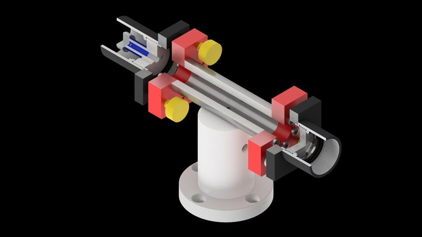
4.1 Quarter cut through the self-built transfer cavity . . . . . . . . . . . . . . . 26
4.2 Schematic of the optics around the transfer cavity . . . . . . . . . . . . . . 28
4.3 Spectrum of the D2 -line of 87 Rb and transmission spectrum of the cavity . 31
4.4 Resonance frequencies of a degenerate cavity . . . . . . . . . . . . . . . . . 33
4.5 Schematic chart of the transfer cavity and laser locking electronics . . . . . 35
4.6 Visualization of the side-lock technique . . . . . . . . . . . . . . . . . . . . . 36
5.1 Photoionization simulation starting in the |40S1/2 i Rydberg state . . . . . . 41
5.2 Photoionization simulation including AOM rise and fall times . . . . . . . . 42
5.3 Photoionization time tPI as a function of the ratio Γec /Ωer . . . . . . . . . . 42
6.1 Experimental pulse sequence for the measurements . . . . . . . . . . . . . . 44
6.2 Photoionization efficiency as a function of the laser power . . . . . . . . . . 45
6.3 Measurement of the Rydberg deexcitation laser Rabi frequency . . . . . . . 46
6.4 Simulated total ac Stark shift of the |6P3/2 i and |51S1/2 i state . . . . . . . 48
6.5 Results of the intermediate state detuning measurement . . . . . . . . . . . 50
6.6 Evaluation of the photoionization cross section . . . . . . . . . . . . . . . . 54
A.1 Circuit of the cavity PID controller . . . . . . . . . . . . . . . . . . . . . . . 61
A.2 Schematic of the TA protection circuit . . . . . . . . . . . . . . . . . . . . . 62
A.3 Technical drawing of the spacer . . . . . . . . . . . . . . . . . . . . . . . . . 64
A.4 Technical drawing of the mirror mount (body) . . . . . . . . . . . . . . . . 65
A.5 Technical drawing of the mirror mount (front plate) . . . . . . . . . . . . . 66
A.6 Technical drawing of the piezo holder . . . . . . . . . . . . . . . . . . . . . . 67
IX1 Introduction
1.1 Rydberg atoms
Rydberg atoms are highly excited atoms with one electron orbiting the ionic core on a
large radius [2]. They are named after the Swedish physicist Johannes Rydberg [3].
Rydberg atoms can be excited optically using narrow linewidth lasers [4]. They exhibit some
interesting general properties that scale with the principal quantum number n. For instance,
S-state Rydberg atoms have an increased lifetime compared to lower-lying states, scaling
with n3 . The lifetime of the |50S1/2 i Rydberg state of 87 Rb is around 141 µs [5] compared
to about 27 ns for the |5P1/2 i excited state [6]. The orbital radius of Rydberg atoms scales
with n2 , and their binding energy follows a n−2 dependence [2], usually resulting in a weak
binding to the ionic core.
This weak binding of the excited electron leads to a large polarizability of Rydberg atoms
that scales with n7 . The van der Waals coefficient C6 scales with n11 [4]. This leads to
strong, long-range interactions of the Rydberg atoms, which shift the Rydberg energy
levels of neighboring atoms, making it impossible to excite two Rydberg atoms within a
certain blockade radius rB at the same time [7–9]. This interesting effect is known as the
dipole-induced Rydberg blockade, scaling with n11 .
Another mechanism is the ion-induced Rydberg blockade dominated by the charge-induced
dipole interaction, scaling with n7 . Due to the giant interactions between Rydberg atoms
and a large sensitivity to external fields, Rydberg atoms have sparked the interest of the
current research.
Along with ions [10], nitrogen-vacancy centers [11, 12] or quantum dots [13–15], Rydberg
atoms show a huge potential for a wide range of applications in the pioneering fields of
quantum information technology, quantum computing or quantum communication [16–21].
Many interesting properties of Rydberg atoms have been studied extensively in the course
of the past 80 years [22]. By exploiting the above-mentioned, basic properties of Rydberg
atoms, significant new discoveries have been made. Only some of them are mentioned in
the following. Rydberg atoms have been analyzed in ultracold quantum gases, leading to
excitations of single Rydberg atoms in a Bose-Einstein condenstate [23]. Two-qubit quantum
gates have been explored [24, 25] and Rydberg atoms have been employed to study nonlinear
quantum optics down to the single photon level [26, 27]. This progress of Rydberg physics
has been closely linked to new developments in laser cooling, atom trapping, and imaging
[28, 29].
11 Introduction In the course of research, homonuclear Rydberg molecules, in which a neutral ground state atom is bound to the Rydberg atom due to the interaction with the Rydberg electron, have become a matter of keen interest, and inspired further inquiry [30–37]. 1.2 Studying ion-atom scattering in the ultracold regime The aim of a new experiment at the 5th Institute for Physics at the University of Stuttgart is to study ion-atom scattering in the ultracold, quantum regime [38]. So far, ion-atom interactions have been studied in the cold regime for different combinations of species [39–49], mainly using Paul traps in combination with a conventional magnetic or optical traps for the neutral atoms. However, due to the micromotion of the ions in Paul traps, the interaction could have been only studied in the essentially classical regime. Until now, the S-wave scattering regime has not yet been reached in any experiment [38]. In the new experiment, either a 6 Li? -6 Li or a 7 Li? -7 Li Rydberg molecule will replace the Paul trap. After the Rydberg molecule has been initialized by photoassociation out of an ultracold atomic cloud, the single lithium Rydberg molecule will be photoionized in order to trigger the ultracold scattering process [38]. The outcome of this process will then be detected with high spatial and temporal resolution using a delay-line detector. To magnify the scattering wavefunction up to a factor of 1000, an ion microscope containing three electrostatic lenses will be used [50]. Rydberg molecules have been chosen, since they offer well-defined starting conditions with only one single Rydberg excitation due to the Rydberg blockade and the tight focus of the respective laser beams. Moreover, ion and atom are already close to each other. To photoionize the Rydberg molecule, a novel V-type photoionization process is employed. In such a V-type scheme, the Rydberg atom gets deexcited into an intermediate state, from where it is photoionized. In contrast to electric field ionization, the photoionization offers high spatial control due to a tight focus of the photoionization beam, and the recoil imparted by the photoionization laser onto the emerging ion is negligible. As the wavelength of the photoionization laser can be tuned directly above the ionization threshold, ultra low-energy ions can be produced, since the electron carries away most of the kinetic energy of the system, and the photoionization allows to minimize the total energy impact onto the ion-atom system. For the Li+ -Li ion-atom system, a photoionization laser which is blue-detuned by maximally 10 GHz from the ionization threshold yields a kinetic energy of the ion that is much smaller than the S-wave scattering limit of the ion-atom system. In order to achieve a diabatic photoionization process for the lithium system (which is to prevent the Rydberg molecule wavefunction from evolving), the timescale is limited to photoionization times on the order of a few ns [38]. The V-type photoionization process can be realized on such a timescale and benefits further from a fast repetition rate. 2
1.3 About this thesis

In the scope of this thesis, the aforementioned V-type photoionization scheme has been
implemented. However, it has been exemplified for 87 Rb. In the future, the experiment will
also feature a lithium oven, and the knowledge gained with the rubidium system can be
employed to set up a new photoionization system for lithium.

1.3 About this thesis

This master thesis will be subdivided into seven chapters. This chapter has already given an
introduction into the background of Rydberg physics and the novel V-type photoionization
scheme. In chapter 2, the theoretical foundations will be outlined. The experimental and
optical setup for the V-type photoionization of 87 Rb will be presented in chapter 3, and
chapter 4 will report on the self-built transfer cavity that is used to frequency-stabilize the
1010 nm photoionization laser. Results of numerical photoionization simulations will be
shown in chapter 5. The experiments that have been performed with the photoionization
laser system will be outlined and analyzed in chapter 6. Chapter 7 will summarize the content
of this thesis, and it will provide an outlook into further research directions. Supplemental
material will be attached in the appendix.

                                                                                             3
2 Theoretical foundations
In this chapter, the theoretical foundations for the mechanisms related to the photoionization
of rubidium described in this thesis will be given. At the beginning, there will be a brief
review of the element rubidium. The second section will be dedicated to the atom-light
interaction, whereas the fundamental theory of optical resonators will be described in the
third section. At last, a short introduction into dipole matrix elements in quantum mechanics
will be given. Further information on specific topics will be provided in the respective
chapters in appropriate detail. For information that is not covered in this thesis, the reader
is referred to literature.
2.1 Physical properties of rubidium
Rubidium (derived from the latin expression rubidus, deepest red) is an alkali metal with
a silver-white apperance [51]. Naturally, the element rubidium consists of two different
bosonic isotopes. 85 Rb is stable and has a natural abundance of 72.17 % compared to 87 Rb
with 27.83 %. In the experiment, the weakly radioactive isotope 87 Rb (with a half-life of
roughly 49 billion years [52]) is used.
As an alkali atom, rubidium has one valence electron. In its 5S1/2 ground state, the ionization
energy EI of a 87 Rb atom is 4.177 127 06(10) eV [53]. The nuclear spin of a 87 Rb atom is
I = 3/2. Due to its positive scattering length, 87 Rb is a suitable element for Bose-Einstein
condensation [54]. Selected properties of 87 Rb are presented in Tab. 2.1 along with their
numeric value and the reference.
87
Tab. 2.1: Physical properties of Rb.
Property Symbol Numeric value Reference
Atomic number Z 37 [51]
Number of nucleons A 87 [51]
Atomic mass m 1.443 160 684(72) × 10−25 kg [55]
Nuclear spin I 3/2 [51]
Ionization limit EI 4.177 127 06(10) eV [53]
52 Theoretical foundations
2.2 Atom-light interaction
This section will introduce the most important principles of atom-light interactions that are
essential in order to fully comprehend the work presented in this thesis. It will outline the
density matrix formalism, the temporal evolution of quantum systems, the fundamentals
of a three-level system, and the ac Stark effect. However, the subjects covered in the
following subsections will provide but a quick overview and will present the notation that
is used consistenly throughout the thesis. For a more comprehensive insight in atom-light
interactions, the reader will find a comprehensive overview of the subject in standard
references such as [56–58].
2.2.1 The atom-light interaction Hamiltonian
A single non-interacting atom with i discrete energy levels |ii with energy eigenvalues
Ei = ~ωi is represented by the Hamiltonian
X
H0 = ~ωi |ii hi| . (2.1)
i
Commonly, the interaction of an atom with a classical light field is dominated by the electric
field component E of the light field that couples to the atomic dipole moment d. In the
dipole-approximation, this interaction is described by the interaction Hamiltonian [59]
HI = −d · E. (2.2)
The electric dipole moment is given by d = −er, where e is the elementary charge and r
denotes the position operator. The atom-light interaction Hamiltonian is composed of both
H0 and HI and given by
HAL = H0 + HI . (2.3)
2.2.2 Density matrix formalism
Whenever a pure state in a quantum system can be described by a single wavefunction
|ψ(t)i, it is possible to define a density operator [60] by the outer product
ρ(t) = |ψ(t)i hψ(t)| . (2.4)
Expanding the wavefunction |ψ(t)i into a complete set of orthonormal basis functions {|ni}
leads to
X
|ψ(t)i = cn (t) |ni (2.5)
n
62.2 Atom-light interaction
and the density operator from Eqn. (2.4) becomes
X X
ρ(t) = cn (t)c∗m (t) |ni hm| = ρnm (t) |ni hm| , (2.6)
n,m n,m
where the elements hn| ρ(t) |mi = ρnm (t) describe the time-dependent matrix elements of
the density operator [56]. The diagonal elements n = m of the density matrix in Eqn. (2.6)
are called populations and the off-diagonal elements n =6 m are referred to as coherences
as they descibe the coherent superpositions of the states |ni and |mi. Due to population
conservation, the normalization condition of the density matrix is Tr[ρ] = 1, where Tr[ρ] is
the trace of ρ.
Since the density matrix formalism is capable of describing both coherent and incoherent
evolutions of atomic ensembles, it will be used within this work in order to describe and
compute the time evolution of the quantum systems [58, 61].
2.2.3 Time evolution of quantum systems
By taking the time derivative of the density operator from Eqn. (2.4), one obtains
∂ρ(t) ∂ ∂
= |ψ(t)i hψ(t)| + |ψ(t)i hψ(t)| . (2.7)
∂t ∂t ∂t
∂
Inserting the Schrödinger equation i~ ∂t |ψ(t)i = H |ψ(t)i and its dual expression into
Eqn. (2.7) results in the von-Neumann equation
∂ρ i
= − [H, ρ] , (2.8)
∂t ~
that describes the time evolution of a coherent quantum system characterized by the density
operator with respect to the Hamiltonian H [58]. However, the full quantum mechanical
description is given by the Liouville-von-Neumann equation
∂ρ i
= − [H, ρ] + L(ρ), (2.9)
∂t ~
a master equation, which also includes incoherent processes such as decay or dephasing
mechanisms that are included in the Lindblad operator L(ρ) [62]. For example, the Lindblad
operator for a decay between two states |ii and |ji at a decay rate Γij is given by
1X
† †
X
†
L(ρ) = − Γij Cij Cij ρ + ρCij Cij + Γij Cij ρCij , (2.10)
2
i,j i,j
†
where Cij = |ii hj| = Cji is a transition operator [61, 63]. The description of dephasing can
be achieved in a similar way that is not presented here.
72 Theoretical foundations
|3i
Γ31 ∆23
|1i
∆12
Γ32
Ω23
Γ12
Ω12
|2i
Fig. 2.1: V-type three-level system. The laser-driven transitions between levels |ii and |ji are
indicated with corresponding Rabi frequencies Ωij . The detuning of a laser with respect to the
atomic transition is marked with ∆ij . Possible decay paths are denoted with Γij . The transition
from |1i to |3i is forbidden by selection rules.
2.2.4 V-type three-level system
In this section, an atomic three-level system is examined. A typical representation of such a
system is the V-type configuration as shown in Fig. 2.1. In the basis of the three states
1 0 0
|1i = 0 , |2i = 1 , |3i = 0 , (2.11)
0 0 1
the Hamiltonian is diagonal, and following Eqn. (2.1) defined as
~ω1 0 0
H0 = 0 ~ω2 0 . (2.12)
0 0 ~ω3
The transitions from |1i to |2i and from |2i to |3i are driven with two laser beams described
by electric fields
1
E12 = E0,12 e−iω12 t + eiω12 t ,
2 (2.13)
1
E23 = E0,23 e−iω23 t + eiω23 t ,
2
with amplitudes E0,12 and E0,23 and angular frequencies ω12 and ω23 , respectively. Both
transitions are far detuned from each other, and the influence of one laser onto the other
transition and vice versa can be neglected.
82.2 Atom-light interaction
Hence, the interaction Hamiltonian according to Eqn. (2.2) becomes
0 −d12 E12 0
1
HI = −d21 E21 0 −d23 E23 , (2.14)
2
0 −d32 E32 0
assuming that the transition from |1i to |3i is forbidden by electric dipole selection rules
∗ . To simplify the evaluation of the Hamiltonian H
and Eij = Eji AL = H0 + HI , it is useful to
perform a transformation into the rotating frame of the laser frequencies, and to apply the
rotating-wave approximation to remove rapidly oscillating terms [57, 64]. In said rotating
frame, the atom-light interaction Hamiltonian reads
−∆12 12 Ω12 0
HAL = ~ 21 Ω∗12 0 1
2 Ω23
, (2.15)
1 ∗
0 2 Ω23 −∆23
where ∆12 = (ω1 − ω2 ) − ω12 and ∆23 = (ω3 − ω2 ) − ω23 are the detunings of the lasers with
respect to the atomic transitions, Ωij = −dij Eij /~ are the Rabi frequencies that express the
coupling strength of the respective transition and Ωij = Ω∗ji . Furthermore, an energy offset
of −~ω2 has been applied making |2i the zero energy ground state of the system.
To obtain the full temporal evolution of the three-level system, one still has to add the
incoherent evolution described by the Lindblad operator. An exact evaluation of Eqn. (2.10)
results in
Γ12 ρ22 − Γ31 ρ11 − 12 (Γ12 + Γ31 + Γ32 )ρ12 − 12 Γ31 ρ13
L(ρ) = − 21 (Γ12 + Γ31 + Γ32 )ρ21 −(Γ12 + Γ32 )ρ22 − 12 (Γ12 + Γ32 )ρ23 (2.16)
1 1
− 2 Γ31 ρ31 − 2 (Γ12 + Γ32 )ρ32 Γ31 ρ11 + Γ32 ρ22
where Γij denotes the decay from |ii to |ji. Using the Liouville-von-Neumann equation (2.9)
it is now possible to describe the dynamics of the considered three-level system [58].
2.2.5 The ac Stark effect
An atom placed inside a monochromatic light field oscillating at an angular frequency ωL is
described by the interaction Hamiltonian
HI = −d · E, (2.17)
where d is again the electric dipole operator and E = 12 E0 e−iωL t + eiωL t is the applied
electric field [58]. In the presence of an oscillating electric field an atomic level experiences
an energy shift, which is called the ac Stark shift (or light shift). It can be calculated using
second order time-independent perturbation theory [65].
92 Theoretical foundations
E
|j 0 i
∆Ej
~ωj |ji
~ωL
~ωi |ii
∆Ei
|i0 i
unperturbed perturbed
Fig. 2.2: Illustration of the ac Stark shift in a two-level system. On the left the unperturbed states
|ii and |ji have an energy difference of ~ωij . A far red-detuned laser beam with (ωij − ωL ) > 0 shifts
the two levels by the same energy.
Since the first order shift with respect to HI vanishes in alkali atoms [66], one can analyze
the energy shift ∆Ei = Ei − Ei0 of a level |ii using
!
X 2 1 1
∆Ei = |hi| HI |ji| + . (2.18)
Ei0 − Ej0 + ~ωL Ei0 − Ej0 − ~ωL
i6=j
Here, Ei0 and Ej0 are the unpertubed eigenenergies of the states |ii and |ji, and the sum
over j considers all transitions from state |ii that are allowed by electric dipole selection
rules. Since the frequency ωL of the light field may be detuned significantly from the
atomic resonance frequency ωij = (Ej0 − Ei0 )/~, the rotating-wave approximation cannot be
applied and hence both co- and counter-rotating terms need to be considered in Eqn. (2.18)
[58, 67, 68].
As an example, Fig. 2.2 shows an illustration of the ac Stark effect for only two states |ii
and |ji. For a red-detunded laser, that is ωij − ωL > 0, the low-lying state |ii experiences a
red-shift whereas the state |ji is shifted towards blue frequencies. The total ac Stark shift is
given by ∆Eac = ∆Ej − ∆Ei .
2.3 Resonator theory
Optical resonators are used in a wide range of applications. Among them are laser resonators
surrounding the gain medium, interferometers, optical filters, spectrum analyzers or optical
frequency standards such as reference cavities [69]. This section will focus on the latter and
will give a theoretical overview on spherical resonators.
In the following, some important general formulae will be presented, the resonator stability
conditions will be outlined and the mode-matching of a laser beam and a resonator will be
illustrated. A brief discussion on the contribution of transversal modes in resonators will
conclude the section.
102.3 Resonator theory
λ
R1 , R1 R2 , R2
L
Fig. 2.3: Schematic drawing of a spherical resonator. The two mirrors with curvatures R1,2 and
reflectivities R1,2 have a distance of L.
2.3.1 Free spectral range and finesse
A spherical resonator consist of two mirrors of reflectivities R1,2 and curvatures R1,2 separated
by a distance L. Such a resonator is schematically depicted in Fig. 2.3. Light of a laser beam
trapped between the two mirrors of this resonator is reflected back and forth. Standing
waves as eigenmodes of the resonator emerge once the condition for constructive interference
λ
q =L (2.19)
2
is met, where q is an integer and λ the wavelength of the light inside the resonator. Using
the relation c = ν · λ with the speed of light c in the respective medium, one obtains the
frequency of the q-th mode as
qc
νq = . (2.20)
2L
The constant spacing of two adjacent modes νq and νq+1 is called the free spectral range of
a resonator [70] and is defined as
c
∆νFSR = νq+1 − νq = . (2.21)
2L
Due to the non-unity reflectivities of the two mirrors, light can enter and exit the cavity.
The transmitted intensity distribution of the resonator as a function of the light frequency
ν is given by
" #−1
2F 2 2
πν
IT (ν) = I0 1 + sin . (2.22)
π ∆νFSR
A detailled derivation for Eqn. (2.22) is given in Ref. [71]. The parameter F is called the
finesse of a resonator. It is defined as the ratio of the free spectral range and the full width
at half maximum (FWHM) of the transmission peaks. It is
√
∆νFSR π R
F= = , (2.23)
νFWHM 1−R
112 Theoretical foundations
1
Normalized intensity IT (ν)/I0
F ≈ 313
0.8 F ≈ 14
F ≈6
0.6
0.4
0.2
0 νq−1 νq νq+1
Resonator mode
Fig. 2.4: Normalized transmitted light intensity IT (ν)/I0 of a spherical resonator as a function of
the resonator mode for three different reflectivities R = R1,2 = {0.60, 0.80, 0.99}. With increasing
reflectivities R the finesse F becomes larger and the width νFWHM of the transmission peaks gets
smaller.
√
where R = R1 R2 is the combined reflectivity of both mirrors. The finesse is a measure for
the quality of a resonator and proportional to the Q-factor in mechanical oscillators [72]. In
Fig 2.4 the spectrum from Eqn. (2.22) is plotted for three different mirror reflectivities.
2.3.2 Resonator stability
There are various types of resonators that use different configurations of concave, convex,
planar or spherical mirrors. Not all combinations provide a stable resonator. This section
will give a quantitative overview on the criteria for the stability of resonators.
A resonator can be treated as a periodic optical system. Unwrapping the resonator presented
in Fig. 2.3 and deconstructing it into a propagation through free space, a mirror, another
propagation, and again a mirror makes it easy to describe the resonator within the ray
transfer matrix formalism.
A detailed consideration of the eigenvalues of the arising matrix in said formalism [73] yields
the stability condition
0 ≤ g1 g2 ≤ 1. (2.24)
The so-called stability parameters gi in above inequality are defined by
L
gi = 1 − . (2.25)
2fi
122.3 Resonator theory
g2
1
1
4
−1
g1
2 1
−1
3
Fig. 2.5: Stability diagram of a resonator. For values g1 and g2 in the shaded regions of the plot
a resonator fulfills Eqn. (2.25) and is stable. There are four special cases pointed out: (1) planar
resonator, (2) confocal resonator, (3) spherical resonator and (4) confocal-planar resonator.
This expression is the general solution for any mirror with focal length fi [74]. The stability
condition from Eqn. (2.24) can be transferred into a stability diagram as shown in Fig. 2.5.
In this figure, there are four special cases of resonators pointed out. Note the spherical
resonator with fi = −Ri /2 and the confocal-planar resonator with R1 = −L and R2 = ∞
[74].
2.3.3 Mode matching of light beams and resonators
All considerations in previous sections have been made under the assumption of plane
waves light fields. However, laser beams are more accurately described as Gaussian beams.
Gaussian beams are the solution of the paraxial Helmholtz equation with axial symmetry.
The electric field distribution of Gaussian beams is described by
2
r2
w0 r
E(r, z) = E0 exp × exp (ikz − iψ(z)) × exp ik . (2.26)
w(z) w2 (z) 2R(z)
The first factor in Eqn. (2.26) describes the amplitude distribution, the second one the
longitudinal phase and the third factor the radial phase of the beam [74]. The beam waist
at position z is described by
s 2
z
w(z) = w0 1 + , (2.27)
zR
where w0 is the minimum beam waist and
πw02
zR = (2.28)
λ
132 Theoretical foundations
is the Rayleigh length. The curvature of the wavefront of the beam is given by
z 2
R
R(z) = z 1 + . (2.29)
z
Furthermore, k is the wavevector and ψ(z) is the so-called Gouy phase [74], which will be
examined more closely in Sec. 2.3.4.
To allow for the best mode matching of the incident laser beam and the resonator, it is
mandatory that the curvatures of the mirrors R1,2 at positions z1,2 match the curvatures of
the Gaussian beam at the same positions z1,2 . Thus, the conditions
2
zR 2
zR
R1 = z1 + , R2 = z2 + with z2 = z1 + L (2.30)
z1 z2
need to apply [75].
2.3.4 Resonance frequencies of a resonator
Gaussian beams as described in Eqn. (2.26) are not the only solution to the paraxial
Helmholtz equation. Another solution is given by Hermite-Gaussian beams, that have a
transversal intensity profile which is described by two sets of Hermite polynomials [76].
The Hermite-Gaussian modes are labelled with TEMlm where l, m ∈ Z and l, m = 0 is the
Gaussian fundamental mode.
The contribution of Hermite-Gaussian modes as well as the previously introduced Gouy
phase ψ(z) change the resonance frequencies of a resonator. In a spherical resonator these
are
∆ψ(z)
νq,l,m = q∆νFSR + (l + m + 1) ∆νFSR , (2.31)
π
where q represents longitudinal modes and l, m label transverse modes [69]. The expression
∆ψ(z) = ψ(z2 ) − ψ(z1 ) is the Gouy phase difference with
z
ψ(z) = arctan . (2.32)
zR
The Gouy phase difference in Eqn. (2.31) collectively shifts the resonance frequencies of a
resonator by a significant fraction of ∆νFSR . Fundamental modes l, m = 0 hence appear at
positions
∆ψ(z)
νq,0,0 = q + ∆νFSR . (2.33)
π
Additionally, higher order modes of a Hermite-Gaussian beam appear in the spectrum of a
resonator.
142.4 Dipole matrix elements
2.4 Dipole matrix elements
This section will give a brief introduction into the quantum mechanical calculation of dipole
matrix elements. A transition between two atomic states |J, mJ i and |J 0 , mJ 0 i is coupled by
the dipole operator d = −er. The dipole matrix element µ = hJ, mJ | d |J 0 , mJ 0 i determines
the coupling strength of said two levels and it arises due to the overlap of the wavefunctions of
levels |J, mJ i and |J 0 , mJ 0 i. Some physical properties such as radiative lifetimes or transition
probabilities can be calculated knowing the quantity of the dipole matrix element [77].
When dealing with angular momenta, it is reasonable to perform a change of basis and
approach arising problems in a spherical basis, where the unit vectors êq are defined by
1
ê±1 = ∓ √ (x̂ ± iŷ) and ê0 = ẑ, (2.34)
2
where x̂, ŷ and ẑ are the Carthesian basis vectors. The expression of the q-th component of
the dipole operator in the new basis is then given by
r
4π q
dq = −er Y (ϑ, ϕ)êq . (2.35)
3 1
Here, Ylm (ϑ, ϕ) are spherical harmonics and q = {−1, 0, +1} labels the three different
polarizations {σ + , π, σ − } of light [78].
The Wigner-Eckart theorem allows to factorize the dipole operator into a reduced matrix
element and an angular contribution, which can be expressed solely in terms of Clebsch-
Gordan coefficients or Wigner 3-j symbols (:::). It is
hJ, mJ | dq |J 0 , mJ 0 i = hJkdkJ 0 i × hJ, mJ |J 0 , mJ 0 ; 1 qi
!
J 0 −1+mJ
√ J0 1 J (2.36)
= hJkdkJ 0 i × (−1) 2J + 1 .
mJ 0 q −mJ
The reduced matrix element hJkdkJ 0 i contains the radial dependence of the dipole matrix
element, while its orientation is fully described by Clebsch-Gordan coefficients [58, 79, 80].
The total angular momentum J = L + S of the atom is a composition of the orbital angular
momentum L and the electron spin S. Since both L and S refer to different Hilbert spaces
and the dipole operator leaves the electron spin untouched, it is possible to further decompose
the reduced matrix element from Eqn. (2.36). Applying the Wigner-Eckart theorem and
using Wigner 6-j symbols {:::} yields
( )
0 L L 0 1
hJkdkJ 0 i = hLkdkL0 i × (−1)J +L+1+S (2J 0 + 1)(2L + 1)
p
. (2.37)
J0 J S
A further decomposition results in
!
0 0 0 −L
√ L 1 L0
hLkdkL i = hnL| er |n L i × (−1) 2L0 + 1 , (2.38)
0 0 0
152 Theoretical foundations
where
Z
0 0 ∗
hnL| er |n L i = µrad = RnL (r)erRn0 L0 (r)r2 dr (2.39)
is the radial matrix element with RnL (r) being the radial wavefunctions with respect to the
quantum numbers n and L [77].
163 Experimental setup
This chapter will provide an introduction into the Rydberg excitation scheme employed in
the experiment and the V-type photoionization scheme implemented in the scope of this
thesis. Moreover, the optical setup of the photoionization laser system (1010 nm) and a
proposed extension of the Rydberg excitation and deexcitation laser system (1020 nm) will
be presented.
3.1 Rydberg excitation and V-type photoionization scheme
To excite atoms to the Rydberg state, a two-photon process is employed using a 420 nm and
a 1020 nm laser in a ladder-configuration. Both lasers have a narrow linewidth on the order
of 25 kHz [81]. The light of the 420 nm laser is σ + -polarized and drives the transition from
the |5S1/2 , F = 2, mF = 2i ground state to the |6P3/2 , F = 3, mF = 3i intermediate state in
87 Rb. The blue laser has a detuning ∆ with respect to the atomic resonance frequency,
which is discussed later. The setup of the 420 nm laser system is described in Ref. [81].
From the |6P3/2 i intermediate state, S- and D-Rydberg states can be adressed using the
1020 nm laser. For S-states σ − -polarized light is used, D-states can be excited with σ +
polarization. Only |nS1/2 i states are considered in this thesis. The wavelength of the
infrared laser can be set to any desired wavelength in the range from 1000 to 1025 nm [82],
which allows to adress many different Rydberg states with principal quantum number n.
More information on the 1020 nm laser system can also be found in Ref. [81].
The excitation scheme as depicted in Fig. 3.1 is called an inverted scheme as the laser with
the smaller wavelength operates on the transition from the ground to the intermediate state
and the infrared laser drives the transition to the Rydberg state. The related normal scheme
utilizes a 780 nm laser to drive the transition |5S1/2 i → |5P3/2 i and a 480 nm laser to get to
the Rydberg state. The inverted scheme has two advantages. Firstly, the available lasers at
1020 nm deliver more optical output power than the 480 nm lasers in the normal scheme [82].
Secondly, the |6P3/2 i state with τ6P3/2 = 112 ns has a much larger lifetime [83] compared to
the |5P3/2 i state with τ5P3/2 = 27 ns [52] and the dipole matrix elements for the transitions
into the Rydberg state are larger [84].
As mentioned above, the transition |5S1/2 , F = 2, mF = 2i → |6P3/2 , F = 3, mF = 3i is
driven off-resonantly with the blue laser being detuned by ∆ = 2π × 80 MHz. Commonly,
this detuning is large compared to the Rabi frequencies of the 420 nm and 1020 nm laser
173 Experimental setup
E
continuum
0
Rydberg state
|nS1/2 i
1010 nm
1020 nm
∆
−E6P3/2 |6P3/2 , F = 3, mF = 3i
420 nm
−EI |5S1/2 , F = 2, mF = 2i
87
Fig. 3.1: Inverted Rydberg excitation and V-type photoionization scheme in Rb. A 420 nm
and a tunable 1020 nm laser in ladder-configuration excite atoms from the |5S1/2 i ground state
to the |nS1/2 i Rydberg state. The blue laser is detuned by ∆ = 2π × 80 MHz with respect to
the atomic resonance frequency to adiabatically eliminate the |6P3/2 i intermediate state. The
Rydberg deexcitation is driven on resonance with the 1020 nm laser and a high power 1010 nm laser
photoionizes the atom.
and large compared to the decay rate of the |6P3/2 i state with Γ6P3/2 = 2π × 1.42 MHz.
Hence, the |6P3/2 i intermediate state experiences only a weak coherent coupling to the
ground and Rydberg state and does not get populated substantially. This is called the
adiabatic elimination of an intermediate state. As a consequence the three-level system can
be treated as an effective two-level system |5S1/2 i → |nS1/2 i with an effective two-photon
Rabi frequency [85]
Ω420 Ω1020
Ωeff = . (3.1)
2∆
Here, Ωi are the Rabi frequencies of the respective lasers. The adiabatic elimination of the
|6P3/2 i state allows for a fast and efficient Rydberg excitation [86, 87].
For the photoionization, a two-photon V-type scheme is used by applying the 1020 nm
and the 1010 nm laser. The 1020 nm Rydberg laser deexcites the atom in resonance with
the |6P3/2 , F = 3, mF = 3i intermediate state using σ − -polarized light. For example, with
a waist w = 5 µm and a laser power of P = 1 mW a deexcitation Rabi frequency of
Ω = 2π × 26 MHz can readily be achieved in a transition from the |51S1/2 i state. The
183.2 Photoionization laser system
tuneable photoionization laser operates at a wavelength of 1010 nm. In Sec. 3.2 the setup of
the photoionization laser system is described. The photoionization rate from the |6P3/2 i
state into the continuum is given by
σλI
Γ= , (3.2)
hc
which is determined by the photoionization cross section σ, the wavelength λ of the pho-
toionization laser and its intensity I [88]. Further information of the photoionization rate
and the treatment of the transition at hand as a decay is given in Sec. 5.1.
The binding energy of the |6P3/2 i state is calculated as E6P3/2 = 2.949 918 69 eV, which
corresponds to a wavelength of
hc
λth = = 1010.295 nm. (3.3)
E6P3/2
The absorption of a photon at this wavelength exactly overcomes the binding energy of
the atom and gently pushes the electron over the ionization threshold. A consideration of
energy and momentum conservation in the emerging electron-ion system yields an electron
energy of
mion
Ee− = Eex (3.4)
mion + me−
after the photoionization, where Eex = E1010 − E6P3/2 is the excess energy, E1010 is the energy
of a photon of the ionization laser, and mion and me− are the masses of the ion and electron,
respectively. Since the mass ratio me− /mion
1, the electron carries away most of the
kinetic energy of the system leaving a low-energy ion. For instance, the kinetic energy of
the electron is Ee− = 132 µeV for a photoionization laser wavelength of λ = 1010.186 nm.
Furthermore, the excess kinetic energy of the ion can be calculated with
me−
Eion = Eex = 0.84 neV, (3.5)
mion + me−
corresponding to a temperature of T = 9.7 µK.
3.2 Photoionization laser system
In this section, the optical setup of the photoionization laser system will be described. A
schematic drawing can be found in Fig. 3.2. The whole setup is placed on a 90 cm × 60 cm
breadboard1 that is mounted on top of the laser table with four 21 cm high stainless steel
posts. This laser table extension is mantled within a cage of opaque plexi glass for reasons
of laser safety and temperature stability.
1
Nexus breadboard B6090L
193 Experimental setup
780 nm to experiment
DLpro 1010 nm
3
250 mm
1020 nm
100 mm
70 mm
wave-
1020 nm meter
1010 nm
shutter
TA
300 mm
AOM
780 nm
1 2
−50 mm 100 mm
mirror λ/2-wave plate photo diode
dichroic mirror polarizing beam splitter optical isolator
adjustable mirror lens fiber coupler
Fig. 3.2: Schematics of the optical setup of the 1010 nm photoionization laser. After the DLpro
laser the shape of the beam is adjusted with an anamorphic prism pair to gain a round beam profile.
The beam is coupled through an optical isolator. Using a λ/2-wave plate and a PBS, 2 mW of the
beam power is guided to a fiber coupler to the wavemeter. 8 mW of the input power is directed to
the cavity branch, where both the photoionization laser and a 780 nm laser are overlapped with the
help of a dichroic mirror and coupled into a polarization-maintaining fiber to the transfer cavity.
The cavity, mode-matching optics and the detection photo diodes (gray box) are set up on the laser
table to give further stability to the cavity. The third branch of the laser (approximately 18 mW)
is coupled into a tapered amplifier (TA) using a cylindrical 2:1 telescope. After the TA the laser
has a power of 2 W. Subsequently, the beam propagates through a cylindrical beam shaping lens,
an optical isolator and is focussed through an AOM and a shutter with the help of a 3:1 telescope.
Behind the third PBS, the beam is coupled into a polarization-maintaining fiber to the experiment.
203.2 Photoionization laser system
The photoionization laser is a Toptica DLpro laser with a wavelength of 1010 nm. An
injection current of 91 mA produces an optical output power of 28 mW. The beam height
of the whole setup is 75 mm. Right after the laser output, an anamorphic prism pair is
used to transform the input beam into a circular-shaped beam. The laser beam is coupled
through an optical isolator2 using two mirrors. At two polarizing beam splitters (PBS 1 and
PBS 2) the beam is divided into three branches. In the following, these three branches are
referred to as wavemeter, cavity and TA branch. The abbreviation TA stands for tapered
amplifier.
The optical power that is deflected into the wavemeter branch can be adjusted with the
λ/2-wave plate in front of PBS 1. Roughly 2 mW are coupled into the fiber connected to a
wavemeter3 . With an adjustable mirror after the fiber outcoupler, the light of the 1020 nm
laser (see Sec. 3.3) from the laser table (see Ref. [81]) can be coupled into the fiber instead
of the photoionization laser in order to avoid unplugging fibers at the input ports of the
wavemeter.
The combination of the second λ/2-wave plate and the PBS 2 branches off about 8 mW into
the cavity branch. With the help of two mirros and another λ/2-wave plate, the 1010 nm
laser is coupled into a polarization-maintaining single mode fiber. In front of the fiber, a
long-pass dichroic mirror4 is placed. This is where the infrared laser is overlapped with a
780 nm laser, which allows for a co-propagation of both lasers through the fiber.
After the fiber, which is outcoupled on the laser table, both laser beams are coupled into
the transfer cavity using two mirrors and a lens with a focal length of 250 mm to fulfill the
mode-matching conditions for the cavity. The cavity is used to perform a transfer-lock from
the 780 nm laser to the photoionization laser. The light transmitted through the cavity of
both lasers is separated with a short-pass dichroic mirror5 and distributed to a photo diode
each. To prevent leakage light from the photoionization laser to reach the photo diode of
the 780 nm laser, a band pass filter6 is installed. The self-built transfer cavity is discussed
in appropriate detail in Ch. 4.
In the TA branch, an aberation-balanced [89] and cylindrical 2:1 telescope magnifies the
photoionization laser beam in one direction to maximize the overlap of the laser beam with
the input facet of the tapered amplifier (TA). The TA itself is seeded with a laser power of
18 mW. An injection current into the TA chip7 of 5.8 A creates an optical output power of
2 W at 1010 nm. After the TA, a 70 mm cylindrical lens is used to correct the beam shape
of the output mode as best as possible. A two-stage optical isolator8 with an isolation larger
than 60 dB prevents reflections into the TA chip [90].
2
Linos FI-980-3SC
3
Burleigh WA-10
4
Thorlabs DMLP950
5
Thorlabs DMSP950
6
Thorlabs FB780-10
7
Dilas TA-1010-2000-CM, facet size 6 × 1.2 µm2
8
Linos FI-980-5TIC
213 Experimental setup
A 3:1 telescope focuses the laser beam through an acusto-optic modulator9 (AOM) and a
shutter10 . The first diffraction order of the AOM (+200 MHz) is coupled into a polarization-
maintaining fiber to the experiment. Due to the diffraction efficiency of the AOM and
the coupling efficiency of the fiber, approximately 500 mW photoionization laser power are
available after the fiber. At PBS 3, the photoionization laser can be overlapped with the
1020 nm Rydberg excitation and deexcitation laser (see Sec. 3.3).
3.3 Rydberg excitation and deexcitation laser system
In this section, an extension for the setup of the 1020 nm Rydberg excitation and deexcitation
laser will be proposed. The major part of the 1020 nm laser system already exists and is
depicted in Fig. 3.7 in Ref. [81].
The main idea of the setup presented in Fig. 3.3 in this work is to overlap three laser beams
to have all lasers for the V-type photoionization process accessing the experiment chamber
through the same viewport. The two Rydberg lasers for the excitation and deexcitation and
the photoionization laser are combined in front of the fiber to the experiment to ensure the
overlap of the beams. The proposed setup is described in the following.
(2) (1)
+80 MHz
1020 nm
1020 nm
3
5 4
AOM
shutter
Fig. 3.3: Proposed optical setup of the 1020 nm Rydberg excitation and deexcitation laser system.
The first 1020 nm beam (1) is guided through a double-pass AOM with a total frequency modulation
of −160 MHz. It is used for the Rydberg deexcitation. The AOM double-pass consists of a lens, a
λ/4-wave plate and a mirror. The second incoming 1020 nm beam (2) is already modulated with
+80 MHz and it is directly coupled into the fiber to the experiment via the shutter and PBS 3 serving
as the Rydberg excitation laser. The zeroth order of the AOM is blocked. The overlap with the
photoionization laser setup in Fig. 3.2 is greyed out in this schematic.
9
Crystal Technology AOM 3200-1117
10
Uniblitz LS3ZM2
223.3 Rydberg excitation and deexcitation laser system
At PBSC 1 in Ref. [81], the first 1020 nm laser beam is picked up11 . The second 1020 nm
beam (+80 MHz) is picked up just before the fiber to the experiment using a flip mirror.
Two periscopes are used to guide the laser beams from the laser table to the setup of the
photoionization laser.
Fig. 3.3 illustrates the suggested setup of the Rydberg lasers on the aforementioned laser table
extension. Light of the 1020 nm beam (1) without frequency shift is transmitted through
PBS 4 and coupled into an AOM in double-pass configuration, leading to a frequency shift
of −160 MHz. This laser is used for the Rydberg deexcitation.
The second 1020 nm laser (+80 MHz) is used for the Rydberg excitation. At a 90:10 beam
splitter (BS 5), the beam is overlapped with the deexcitation beam and coupled into the
fiber to the experiment. A shutter is utilized to block the laser beams.
Since the 420 nm laser is detuned by +80 MHz, the combined frequency shifts of the Rydberg
excitation laser (−160 MHz) and the Rydberg deexcitation laser (+80 MHz) ensure that
the Rydberg deexcitation laser couples the Rydberg state |nS1/2 i resonantly to the |6P3/2 i
state.
11
Note the different notation PBSC for polarizing beam splitter cubic, which is used in Ref. [81]
234 Self-built transfer cavity
In this chapter, the self-built transfer cavity will be introduced, and the specific requirements
for the cavity will be sketched out. A novel transfer cavity design will be presented and
explained. The developed theoretical mode-matching considerations will be continued and
applied to the cavity at hand. Finally, the self-built cavity will be characterized and the
frequency and length stabilization of both the involved lasers and the cavity will be presented.
A tutorial on how to easily adjust the cavity and couple light into it can be found in appendix
A.4.
4.1 Requirements
The principal purpose of the cavity is to perform a transfer lock from a laser with wavelength
780 nm to a laser with wavelength 1010 nm. Therefore, a cavity with an active length-
stabilization mechanism is needed. This is realized making use of a piezo actuator to keep
the cavity at constant length. Due to previous experiences of the institute with plano-concave
cavities, this configuration is also used for the cavity presented in this thesis.
In order to produce slow ions and impart as little energy as possible onto them during
the photoionization process, the 1010 nm photoionization laser should be tuned close to
the ionization threshold of the 87 Rb atoms. Therefore, a free spectral range of around
∆νFSR ≈ 1 GHz is required. Rearranging Eqn. (2.21) would yield a desired length of the
cavity of L = c/(2∆νFSR ) = 150 mm. However, the cavity length is chosen to be L = 160 mm
resulting in a free spectral range of ∆νFSR = 937.5 MHz. The reason for the slightly longer
cavity is the degeneracy of fundamental and Hermite-Gaussian modes that would appear in
a cavity of 150 mm length. This will be briefly discussed in Sec. 4.4.2.
Since a laser linewidth on the order of tens of MHz is sufficient for the photoionization
process, no high finesse cavity is needed. Therefore, this aspect is not considered in the
conception of the transfer cavity.
254 Self-built transfer cavity
piezo holder
fine tuning screws
plane mirror M1
spacer
mirror mount
(front plate)
piezo actuator
lens tube
mirror mount
(body)
concave mirror M2
retaining ring
mounting post
Fig. 4.1: Quarter cut through a rendered image of the self-built transfer cavity. The individual
parts of the cavity are labelled within the figure.
4.2 Design and realization
The cavity, as depicted in Fig. 4.1, is designed in a plano-concave configuration of two
commercially available mirrors. The plane mirror M1 is a broadband laser mirror by Lens-
Optics12 with a diameter of 12.5 mm to cope with both laser wavelengths. It is made of
a BK7 glass substrate and has a nominal reflectivity R1 > 99.6 % in the range of 760 to
1064 nm due to the high reflectivity coating. The curvature of this mirror is R1 = ∞. Mirror
M2 is a dielectric-coated concave mirror by Thorlabs13 with a diameter of 25.4 mm and
a focal length f2 = 100 mm. It has a curvature of R2 = −2f2 = −200 mm. The average
reflectivity over the whole coating range from 750 to 1100 nm is specified as R2 > 99.0 %.
The stability parameters of the two mirrors according to Eqn. (2.25) are g1 = 1 and g2 = 0.2,
respectively. Therefore, the cavity is considered stable, as the inequality from Eqn. (2.24)
0 ≤ g1 g2 = 0.2 ≤ 1 (4.1)
is fulfilled. A cavity with one mirror of curvature R1 = ∞ is considered a special case of a
spherical resonator [69]. Hence, all theoretical studies from Sec. 2.3 are applicable to the
cavity at hand.
12
Lens-Optics M760-1064/12.5 with HR760-1064 nm/0-45°, s+p-Pol. coating
13
Thorlabs CM254-100-E03-SP (backside polished)
264.2 Design and realization
The concave mirror is mounted inside a lens tube14 and fastened with a retaining ring. On
the opposite side of the cavity, the plane mirror is glued onto a piezo ring actuator with
epoxy resin. The piezo actuator itself is glued to a custom-made stainless steel piezo holder
that comprises feed-throughs and a strain relief for the piezo cables. The whole assembly is
built into another lens tube15 and fixed in place with a retaining ring.
The front plates of two commercially available mirror mounts16 are provided with threads17
and the previously mentioned lens tubes are screwed into them. Both mirror mount bodies
are provided with one through bore each, matching the inner diameter of the spacer tube.
The two aluminium mirror mounts are screwed to a stainless steel tube18 with an inner
diameter of 13 mm and an outer diameter of 25 mm that serves as a spacer between the
mirrors. In its center, the spacer is screwed onto a stainless steel mounting post19 . Technical
drawings of the parts are provided in appendix A.5.
The piezo actuator used in the cavity is a multilayer stack ring actuator20 with six stacks
and a nominal travel range of 11 µm. It can be operated in a voltage range from −20 to
100 V.
There are numerous advantages of this cavity design. The tilting of both mirrors with
respect to the optical axis of the laser beam inside the cavity can be adjusted using the
fine tuning screws on the mirror mounts. Moreover, by inserting additional retaining rings
into the lens tubes, the longitudinal position of both the concave and the plane mirror can
be altered and the free spectral range of the cavity can be modified. Moreover, the lens
tubes containing the mirros can easily be dismantled. This proves to be useful for a rough
adjustment of the laser beam through the cavity. More details on adjusting the cavity are
given in appendix A.4. Furthermore, as the concave mirror is not glued into the cavity as
in previous designs of the institute, it can simply be replaced by another mirror making it
possible to alter properties such as the finesse of the cavity.
The presented design proves to be quite stable and the length of the cavity can actively
be stabilized for over 24 hours. Apart from the spacer, all cavity parts are commerically
available, which cuts production costs.
Moreover, several transfer cavities of the very design explained in this thesis are already
recreated within the institute. Due to the arbitrarily adaptable components of the cavity
and the modular design, a wide range of different properties can be achieved.
14
Thorlabs SM1L10
15
Thorlabs SM1L15
16
Radiant Dyes MDI-2G-3000
17
Done by the mechanics workshop of the Physics Institutes of the University of Stuttgart
18
MiSUMi PIPS25-6-500
19
turned down Thorlabs P75/M
20
PI ceramic P-080.341
27Sie können auch lesen