Reinforcement Learning in Decentralized Multi-Goal Multi-Agent Settings - IAS TU Darmstadt
←
→
Transkription von Seiteninhalten
Wenn Ihr Browser die Seite nicht korrekt rendert, bitte, lesen Sie den Inhalt der Seite unten
Reinforcement Learning in
Decentralized Multi-Goal
Multi-Agent Settings
Reinforcement learning in dezentralisierten Szenarien mit mehreren Zielen und Akteuren
Master thesis by David Rother
Date of submission: May 7, 2021

1. Review: M.Sc. Fabio Muratore
2. Review: Prof. Dr. Jan Peters
Darmstadt
Erklärung zur Abschlussarbeit
gemäß §22 Abs. 7 und §23 Abs. 7 APB der TU Darmstadt

Hiermit versichere ich, David Rother, die vorliegende Masterarbeit ohne Hilfe Dritter und
nur mit den angegebenen Quellen und Hilfsmitteln angefertigt zu haben. Alle Stellen, die
Quellen entnommen wurden, sind als solche kenntlich gemacht worden. Diese Arbeit hat
in gleicher oder ähnlicher Form noch keiner Prüfungsbehörde vorgelegen.
Mir ist bekannt, dass im Fall eines Plagiats (§38 Abs. 2 APB) ein Täuschungsversuch
vorliegt, der dazu führt, dass die Arbeit mit 5,0 bewertet und damit ein Prüfungsversuch
verbraucht wird. Abschlussarbeiten dürfen nur einmal wiederholt werden.
Bei der abgegebenen Thesis stimmen die schriftliche und die zur Archivierung eingereichte
elektronische Fassung gemäß §23 Abs. 7 APB überein.
Bei einer Thesis des Fachbereichs Architektur entspricht die eingereichte elektronische
Fassung dem vorgestellten Modell und den vorgelegten Plänen.

Darmstadt, 7. Mai 2021
                                                                   David Rother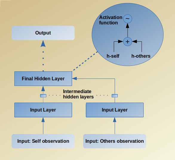
Abstract

Multi-Agent Reinforcement Learning is a trending research topic in many fields such as
robotics, distributed control and economics. Many real-world Multi-Agent tasks are to
complex to be solved by simple rule based systems. Instead, multi-agent reinforcement
learning aims to find solutions through interaction with the environment it is placed
in. However, with AI being increasingly interwoven in our lives, research needs to not
only find good solutions for the one using it, but do so in a socially acceptable manner.
The contribution of this thesis to support efforts in this direction are threefold. First, we
create a novel scenario, where a test of social skill is singled out to measure how well
an algorithm does in that regard. Second, we extend the policy gradient method PPO to
incorporate a social component in its gradient by using the theory of mind concept from
psychology, developing a new algorithm DM3 that takes ideas from the related algorithm
CM3. To compute influence on other agents, an agent takes their perspective and imagines
the impact of its actions by modeling their thought process as its own, leading to a social
understanding of the situation. The last contribution is the incorporation of additional
metrics beyond the sum of rewards, the utilitarian measure. Using different metrics,
invented in the field of social economics, allows one to gauge different properties of the
resulting behavior when evaluating cohabitating artificial agents. We can show that the
newly created scenario distinguishes between social and non-social behavior through
examination of the expected social behavior. Our algorithm DM3 manages to learn in
a social manner, whereas PPO does expectedly not. However, the gained capabilities
come at the cost of local performance power because the algorithm gets stuck in worse
local optima. The additional metrics highlight differences in social capabilities and help
identify where an algorithm performs poorly because of worse local optima and where
the algorithm does not learn social behavior.
Zusammenfassung

Reinforcement Learning mit mehreren Akteuren ist ein aktuelles Forschungsthema in
Robotik, verteilten Steuerungssystemen, Wirtschaft und anderen Forschungsfeldern. Viele
Aufgaben, die mehrere Akteure involvieren, sind zu komplex um sie mit einem Regel
basierten System zu lösen. Stattdessen findet Reinforcement Learning Lösungen durch
Lernen. Da Künstliche Intelligenz (KI) immer weiter in unser Leben eindringt ist es not-
wendig, dass die KI der Zukunft nicht nur ihre Aufgabe löst, sondern dies auch mit einem
sozialen Bewusstsein macht. In dieser Thesis unterstützen wir Forschungsanstrengungen
in dieser Richtung auf drei Art und Weisen. Wir stellen eine neue Lernumgebung für
mehrere Akteure vor, in der wir explizit auf soziales Verhalten testen und dabei andere
Einflussfaktoren möglichst eliminieren. Darüber hinaus erweiteren wir die policy gradient
Methode PPO und inkorporieren soziale Aufmerksamkeit in das Lernverfahren. Dabei
greifen wir auf die Theory of Mind aus der Psychologie zurück, um unser Vorgehen zu
motivieren, und entwickeln einen neuen Algorithmus DM3, der Ideen von dem Algorith-
mus CM3 übernimmt. Um den Einfluss auf andere Akteure zu berechnen, nimmt ein
Akteur die Perspektive eines anderen ein und modelliert den Gedankenprozess seines
Gegenübers als würde er ihn selbst erleben. Dies erlaubt ihm einzuschätzen, welche
Auswirkungen die eigenen Aktionen auf andere haben werden und führt dadurch zu
einem sozialem Verständnis der Situation. Als letztes erweitern wir die Evaluation um
bekannte Metriken aus dem Bereich der Wohlfahrtsökonomik. Indem wir andere Metriken
außer der Summe der Einkommen verwenden, das utilitaristische Prinzip, können wir
unterschiedliche Aspekte des gelernten Verhaltens beurteilen. Wir zeigen, dass unser neu
geschaffenes Szenario eine Unterscheidung von sozialem Verhalten und nicht-sozialem
Verhalten erlaubt. Unser Algorithmus DM3 schafft es, soziales Verhalten zu lernen in
diesem Miniaturbeispiel, während PPO dies nicht kann. Jedoch verschlechtert sich von
DM3 die Performanz die eigene Aufgabe zu lösen, da der Algorithmus zu einem lokal
schlechteren Ergebnis konvergiert. Die zusätzlich angewendeten Metriken unterstreichen
die Unterschiede in den erworbenen sozialen Fähigkeiten und helfen zu identifizieren
an welcher Stelle die Algorithmen aufgrund mangelndem sozialen Verhalten oder einem
suboptimalem Lösungsverhalten bei der eigenen Aufgabe schlecht abgeschnitten haben.
Contents

1. Introduction                                                                               2

2. Related Work                                                                           5
   2.1. Single Agent Learning . . . . . . . . . . . . . . . . . . . . . . . . . . . . . 5
   2.2. Multi Agent Learning . . . . . . . . . . . . . . . . . . . . . . . . . . . . . . 13
   2.3. Evaluation of Reinforcement Learning Algorithms . . . . . . . . . . . . . . 17

3. Methodology                                                                               19
   3.1. Environment . . . . . . . . . . . . . . . . . . . . . . . . . . . . . . . . . .      20
   3.2. Evaluation . . . . . . . . . . . . . . . . . . . . . . . . . . . . . . . . . . . .   21
   3.3. Multi-Goal Multi-Agent Setting . . . . . . . . . . . . . . . . . . . . . . . .       22

4. Experiments                                                                            30
   4.1. Simulation of Urban Mobility (SUMO) . . . . . . . . . . . . . . . . . . . . 30
   4.2. Cooperative Navigation . . . . . . . . . . . . . . . . . . . . . . . . . . . . . 35
   4.3. Social Navigation . . . . . . . . . . . . . . . . . . . . . . . . . . . . . . . . 41

5. Discussion                                                                                49

6. Outlook                                                                                   51

A. Hyperparameter Configurations                                                              58

B. Results Tables                                                                            59

                                                                                              1
1. Introduction
Artificial Intelligence (AI) and machine learning are increasingly adopted not only in
different business domains but also in all different areas of research, such as physics,
chemistry, biology and many more. Those systems are often used to either predict, vi-
sualize our explain some form of data or learn control of robots. Usually, problems are
solved using supervised or unsupervised learning algorithms. However, for challenges
with a system or an agent that can interact with its environment reinforcement learning
solutions may be deployed, as for example in control tasks. Since the advent of Deep
Reinforcement Learning (DRL), by combining RL with deep learning, RL has gained
popularity equally among researchers and media. In 1997 TD Backgammon was the first
successfull application of RL in the game Backgammon [52, 51]. The first milestone that
gained wider attraction was the super-human performance of a DRL agent in Atari games
[31]. Thereafter, multiple other impressive challenges like mastering the board game of
GO have been tackled [47]. Other hard tasks were approached soon after with Dota 2
playing bots by openAI [33]and Starcraft II bots by DeepMind [55]. An ever emerging
topic in RL research are systems with multiple agents. These systems are relevant for
many fields, such as behavioral sciences, control and optimization, economics, robotics
and many more. Expanding single agent RL to multiple agents entails new problems to
be explored [1].
Multi Agent Reinforcement Learning (MARL) is garnering more attention in recent times.
In MARL agents can either be cooperative, competetive or employ mixed behavior without
a clear social status of agents to one another with both friends and foes explicitly defined.
Most studied scenarios are cooperative scenarios, e.g. common ressource allocation [35]
or traffic control [4], and competetive games. In competetive games agents do directly
compete against each other and the most common setting are multiplayer games [52,
47]. Mixed games are even more complex, where an agent has both friends and foes as
for example in team games [33, 55]. But agents still have to find a globally satisfying
solution, which is the same for all agents on a team. However, in those scenarios agents
are explicitly interested in maximizing a team reward and/or rewards of foes are directly
2coupled to form a zero-sum game. Zero-sum games feature opposing players, where the
sum of values of each player is zero. Moreover, the advantage of one player is in total the
same quantitative disadvantage of the other player(s).
There are many different kinds of roblems in MARL and often simplifying assumptions
are required. For example from a learners local perspective the problem becomes non
stationary when other agents learn concurrently and taking the joint action space into
account results in issues regarding scalability [21]. Another issue in MARL is the need for
definition of the learning goal, which could be finding a Nash Equilibrium or the stability
of the policy or a suitable adaptive strategy given a fixed class of other agents [61].
In this work, we look into cooperation of multi agent systems with the possible extension
of human interaction. In the case of multi agent systems, we do not use precomputed
strategies or explicit communication. Currently, most settings concentrate on a single
cooperative goal, where agents need to learn to overcome certain hurdles to achieve
some globally optimal reward. A popular branch of these problems are sequential social
dilemmas, where cooperation is hard to achieve because agents need to learn to not exploit
others as this leads to a local optimum in the reward space [24, 42, 2]. To go even further,
we want to shift the focus away from cooperation and competition, where an action is
beneficial to both or bad for the competitor but beneficial for the own agent.
A rather unexplored area of MARL are coexistence scenarios. In those scenarios multiple
agents act in the same environment but the reward of the agents is not linked to other
agent’s rewards. Each agent has one of many possible goals during an episode and tries to
achieve it, obtaining only local observations and rewards. Coexistence scenarios expand
on the current landscape of mainline MARL work, embedding potentially cooperative
or competetive work into broader real world scenarios, where there might exist other
unrelated agents. Coexistence scenarios in the real world are particularly relevant when
unplanned interaction between multiple agents happens. These situations can happen in
shared workspace environments, such as factories, shared open spaces like roads with
multiple vehicles navigating ,or crowds, where people avoid collisions as good as possible.
The goal of each agent is to maximize its own reward but also maximize the other agent’s
reward if there is no negative impact on its own reward. This introduces an interesting
trade-off because the agents may cooperate but also have to compete potentially for
limited ressources. Since each agent is considered an individual and independent entity
we aim to develop a decentralized learning system.
Current MARL tasks require mostly cooperation and only few even have multiple goals for
different agents, where no explicit cooperation is needed. Additionally, most environments
can be solved, when maximizing for the sum of rewards for all agents such that all agents
arrive at satisfying solutions locally. In contrast, we introduce new multi goal multi agent
scenarios in the multi agent particle environment [29], in which agents share space and
3have to avoid collisions to reach their individual goals.
Logically following, the evaluation of MARL systems with multiple selfish agents in coexis-
tence scenarios needs additional metrics to evaluate what constitutes a good result. In
coexistence scenarios the evaluator might not only be interested in how well the average
of all agents performed but is concerned about other things such as fairness as well. Social
welfare functions from the field of economics and sociology are promising candidates in
that regard [6, 19]. In these fields measures of wealth of a group of humans or agents in
our case exist that take into account the wealth (in reward) for single agents in contrast to
the overall wealth. This allows us to do a richer evaluation and comparison of algorithms
beyond standard measurements.
In this thesis we contribute a novel way to learn in decentralised scenarios, using a credit
mechanism in reinforcement learning and introduce new environment scenarios alongside
a deeper evaluation, by using additional metrics.
The remaining part of the thesis is structured as follows. The next chapter introduces
related work and begins with the foundations of reinforcement learning in single agent sce-
narios. Afterwards, various approaches multi-agent reinforcement learning are presented
and ideas from psychology are described. The third chapter elaborates our approach to
learning, as well as ideas for better evaluation and why new tasks are needed in social
reinforcment learning settings. The fourth chapter contains all experiments. Alongside
the experiments all results are presented and discussed. In the last chapter we give an
overarching discussion and summary of all results and conclude our work in an outlook.
42. Related Work
In this Chapter we introduce the foundations of reinforcement learning in single and multi
agent settings as well as evaluation methods for RL systems. We start with definitions of
reinforcement learning and present algorithms in deep reinforcement learning as well as
various concepts of deep learning. We explore methods of single-agent RL and continue
by explaining different multi-agent RL settings. The concluding part will explain other
MARL methods and how the existing methods relate to our work.
2.1. Single Agent Learning
The basic problem to encounter in reinforcement learning is to control the actions of
a single agent in a stationary environment without other agents or agents with fixed
policies.
2.1.1. Reinforcement Learning
Reinforcement learning is a method in machine learning with which an agent (AI)
adapts its behavior through reinforcement, reward or punishment, when interacting
with an environment [49]. The Agent tries to maximize its reward and adopts a reward
driven behavior [3, 32, 61, 21]. RL can be formulated as a Markov Decision Process
(S, A, R(st , at , st+1 ), P (st+1 |st , at ), γ), where 0 ≤ γ ≤ 1 is the discount factor, which re-
duces the value of the rewrd collected in future states, and t denotes the current time
step. A is the set of actions an agent may take and S is the set of states an agent can be
in, including the subset of inital states. R is a reward function that maps a state, action
and the following state to a scalar reward and P is the State transition function that maps
a state action pair to a state distribution.
The action choice of an agent follows a policy π. In general, the policy π is a mapping
5from states to a probability distribution over actions: π : s ↦→ p(A = a|s). We can compute
the return G of a single episode as
T
∑︂−1
R= γ t rt+1 ,
t=0
where rt+1 is the reward collected at time step t+1. The goal is to maximize the expectation
of the reward for all episodes from each state given a policy, yielding the optimal policy
π∗
π ∗ = argmax E[R|π]. (2.1)
π
Given the basic formulation of MDPs and the key optimization problem we next introduce
the most common approaches for solving tasks with RL.
Value Functions
A value function is a mapping between any state our agent can be in and a real valued
scalar. It describes the expected reward when starting in a state s and taking actions
according to the policy π. Therefore, the value function is defined as
[︄ ∞ ]︄
∑︂
V π (s) = E[R|s, π] = Eπ γ t rt+1 |st = s .
t=0
Similarly to the optimal policy π∗ we can formulate an optimal value function
V ∗ (s) = max V π (s), ∀s ∈ S.
π
Having either the optimal value function or the optimal policy automatically yields the
other one, since we could always pick the action that maximizes the expected return in
any situation. Since we do not have either but rather try to learn the optimal policy or the
optimal value function we introduce another function. The state-action-value function
allows us to compute the expected rewards for each action we can take for each state
action pair (a, s). In other terms the function describes the quality of taking an action a in
state s and is accordingly named the quality function or short Q-function. The Q-function
is defined as
6Qπ (s, a) = E [R|s, a, π] .
Both the value and Q-function depend on the states and available actions because some
states may be intrinsically better than others, such as a winning position in a board game.
But they also depend on the policy since even in a favorable state a bad policy may yield
bad returns.
The last notion we want to introduce is the one of advantage [23, 15]. Advantage aims
to compute the difference of taking any action versus taking an action according to the
current policy. Thus, we get a notion of better or worse with respect to our current policy.
The advantage function is defined as
Aπ (s, a) = Qπ (s, a) − V π (s).
We can deduce that an advantage is positive if Qπ is bigger than V π and a negative vice
versa. Intuitively, we can improve our policy by making actions more likely that have an
advantage over the actions chosen by our current policy.
Given the mathmatical foundation of value, quality and advantage the goal is to solve for
the optimal solution. To this end, we reformulate our problem in a recursive setting, where
the value of our function depends on the recursive application of itself. This paradigm is
known as dynamic programming [5] and it allows us to rewrite the value and Q-function
as their corresponding Bellman equations
∑︂ ∑︂
V π (s) = p(s′ |s, a) r(s, a, s′ ) + γ V π (s′ ) ,
[︁ ]︁
π(s, a)
a∈A s∈S
[︄ ]︄
∑︂ ∑︂
π ′ ′ ′ ′ π ′ ′
Q (s, a) = p(s |s, a) r(s, a, s ) + γ π(s , a )Q (s , a ) .
s′ ∈S a′ ∈A
Since we assume the Markov property, the Bellman equations can be proven to converge
to the best policy with Q-learning [57]. Q-learning tries to learn the Q-function for a
given MDP, that is it estimates the value of state-action pairs. The optimization process
then usually consists of two alternating steps, policy evaluation and policy improvement.
But the major drawback of dynamic programming is that it can only be used if the
dynamics of our MDP are fully known. To add to that, the computational complexity
rises exponentially, also known as the curse of dimensionality, if the number of states
7and state-action pairs gets higher, rendering the algorithm useless for most real world
applications. If the environment is a priori unknown to the agent, one needs to explore
it to get estimates of the V and Q functions. Since bootstrapping value functions using
dynamic programming methods is infeasible, we instead use Monte Carlo methods where
we estimate the expected return of being in a state. This is done by averaging the return
from many different rollouts of our current policy. Thus, we can estimate the value given
a state s and a policy π as
M
1 ∑︂ i
V π (s) ≈ R,
M
i=1
where M is the number of rollouts from state s and Ri is the Return of the i’th rollout.
The main drawbacks of this formulation are the need of episodic MDPs and a sufficient
level of exploration. A lack of exploration may lead to missing the optimal solution and
the agent may be stuck not solving the task or simply not getting out of a local optimum.
This problem is also known as the eploration exploitation dilemma. If the agent explores
too much the evaluated policy simply becomes close to a random policy and does not
yield useful behavior or converge to any coherent behavior. Likewise, if we only select
actions using our current policy the agent might never explore areas of our environment
or action sequences that would improve the final return, thus, never actually reaching
the global optimum. Two possible solutions to the exploration problem are ϵ-soft policies
and the Softmax action selection method. ϵ-soft in the simplest case is ϵ-greedy, where we
select the action according to our policy with a probability of 1 − ϵ and select otherwise
randomly one of the other actions. In practice one starts with a high ϵ value so that many
random actions are taken at the beginning of learning, basically aquiring knowledge of
the world. Later on with lower values the policy starts to exploit this knowledge to find
the optimal solution. In the case of Softmax action selection each action has a probability
of being assigned based on its relative Q-value to all other actions. When using a softmax
distribution one can adjust the "temperature" over time, which adjusts the entropy of
the action distribution. This allows to introduce simulated annealing, which for a slow
enough annealing process guarantees convergence. However, epsilon greedy methods can
be applied universaly to all policy methods to establish sufficient exploration.
In general, to deal with exploration there are two different types of methods available. The
first are on-policy algorithms, where SARSA [40] is a common example using temporal
difference learning. With on-policy methods we create some episodes with our current
policy and use some form of ϵ-soft algorithm to ensure exploration. Second are off-policy
8algorithms, which use a behavioral policy to generate episodes. The behavioral policy is a
different policy from the learned policy. The advantage of off-policy learning is that we
can target the search to more promising areas of the state-action space for example by
using expert generated policies. The disadvantage in that case is that we will not explore
states that the behavioral policy never visits, thus missing potentially better solutions.
Policy Gradients
Instead of learning the value of states there is another learning paradigm in reinforcement
learning called policy search. We learn the policy and maximize (2.1) directly. We do that
by maximizing the expected returns over all trajectories generated by our current policy.
Therefore the objective function becomes
[︄ T ]︄
∑︂
J(θ) = Eτ ∼ρθ [R(τ )] = Eτ ∼ρθ γ t r(st , at , st+1 ) ,
t=0
where τ = (s0 , a0 , s1 , a1 , ..., sT , aT ) is a trajectory generated by our policy and sampled
from the distribution ρθ with θ being the parameters of our policy. In policy gradient
approaches the main idea is to take the gradient of the objective function with respect to
the policy parameters [36]. Updates are then straightforward and using gradient ascent
we obtain the update rule
θnew = θold + η ∇θold J(θold ).
The REINFORCE [58] algorithm estimates the gradient as
∇θ J(θ) = Eτ ∼ρθ [∇θ log ρθ (τ ) R(τ )]. (2.2)
The estimate is Monte Carlo sampling as we take the average of the reward-weighted
log-likelihood of a trajectory. Because we use the empirical returns of each trajectory in
the gradient computation the variance of the gradients is usually very high. We can lower
the variance by introducing a baseline and subtract it from the empirical return. To do
so different algorithms have been proposed that also extend the system to actor-critic
methods, which will be discussed in the deep reinforcement learning section. Policy
gradient methods have a wide array of advantages. Since the formulation does not
9rely on knowing the dynamics of the MDP they are inherently model-free and we do
not need to know about task or reward models. Furthermore, policy gradient methods
are easily applicable to continuous action spaces in contrast to value based methods.
Other advantages are that policy gradient methods empirically have better convergence
properties than Q-learning methods and are generally more stable [10], they are effective
in high dimensional action spaces and they learn stochastic policies. Disadvantages that
one has to face are the inefficient learning of policies through poor sample efficiency, the
convergence to local optima instead of the global one and that the evaluation of the policy
gradient has a high variance.
2.1.2. Deep Reinfocement Learning
Deep Reinfocement Learning (DRL) and especially the use of Convolutional Neural Net-
works (CNN) [26] have made RL methods viable for high dimensional state-action space
problems. Additionally, Recurrent Neural Networks (RNN) [39] and Long-Short Term
Memory (LSTM) [22] architectures make it possible to apply DRL algorithms to problems
with temporal dependencies between states. In this section we present the advances in
Deep Reinforcement Learning (DRL) and mention how the algorithms address different
challenges encountered in the base formulation of RL.
Value Based
The first succesfull application of DRL with a value based approach was the DQN algorithm
[30]. DQN solves two prominent problems, the correlation of inputs and outputs that
arises because succeeding states are not independent, violating the assumption that states
are independent and identically distributed and the non-stationarity of the target Q-values.
These issues are solved with two seperate mechanisms in DQN. The first is an Experience
Replay Memory (ERM) that stores transitions of many runs. Then, training is done on a
random batch sampled from the ERM. The other proposal was the use of a target network
that computes the target Q-values and is frozen over many episodes. It is only updated very
infrequently, allowing the Q-network to learn stationary target values and thus converging.
While ERM and target networks have an overall positive effect, their use slows down
learning by a significant margin and increases sample complexity. To aleviate those
problems several modifications have been proposed, such as double Q-learning [54],
prioritized experience replay [43], duelling networks [56] working with an advantage
10function or a recurrent version DRQN [18] that is able to tackle POMDPs thanks to an
LSTM [22] layer.
Policy Gradient Based
In recent years policy gradient methods in conjunction with DNNs have garnered a lot of
interest in the research community and much progress has been made on the algorithmic
side such as DDPG [48], TRPO [46], PPO [45] and PPG [9]. As mentioned earlier we can
estimate the policy gradient as in Eq. (2.2). According to the policy gradient theorem we
can rewrite this equation in terms of single transitions instead of complete trajectories as
N T T
1 ∑︂ ∑︂ ∑︂ ′
∇θ J(θ) ≈ ( ∇θ log πθ (st , at ) γ t −t r(st′ , at′ , st′ +1 )),
N ′
i=1 t=0 t =t
where additionally the concept of causality is introduced. Because the future reward does
only depend on the reward of future states we simply take the sum of the rewards of
future states, which is the definition of the Q-function. Following this notion Sutton et al.
[49] showed that we can rewrite the gradient of the objective function as
∇θ J(θ) = Es∼ρθ ,a∼πθ [∇θ log πθ (s, a) Qϕ (s, a))],
where a function approximator Qϕ is introduced to estimate the Q-function. The resulting
architecture is actor-critic as we have a policy πθ (s, a) and a critic Qϕ (s, a).
So far the policy gradient is strictly on-policy as we are only allowed to use samples
generated by the current policy. This restriction arises because the data distribution is
dependent on the policy and becomes non stationary as the policy changes. An important
concept to overcome this issue is importance sampling. We can rewrite our objective
function in terms of a behavior policy b and the current policy θ and obtain
ρθ (τ )
J(θ) = Eτ ∼ρθ [R(τ )] = Eτ ∼ρb [ R(τ )],
ρb (τ )
where the ratio ρθ (τ )/ρb (τ ) is the importance sampling weight. It controls how much we
learn from generated trajectories by decreasing importance of trajectories that have a
much higher probability to be generated by the behavior policy than the current policy.
11General Advantage Estimate
An important aspect to make Policy gradient based methods more stable is the Generalized
Advantage Estimate (GAE) [44]. GAE adresses the bias/variance trade-off in machine
learning. In reinforcement learning we get a small bias in the return term of the advantage
formulation, if we rely on real rewards, that is the general return rollout of the trajectory.
If we instead take estimates like the TD error
δt = rt+1 + γV π (st+1 ) − V π (st )
we get a high bias but small variance leading to a more stable gradient that in return may
be more incorrect due to the bias. Schulman et al. takes the n-step advantage
n−1
∑︂
Atn = γ k rt+k+1 + γ n V π (st+n+1 ) − V π (st )
k=0
and instead of choosing a concrete n they reformulate the GAE as
∞
GAE(γ,λ)
∑︂
At = (1 − λ) (γλ)l δt+l , (2.3)
l=0
where δt = rt+1 + γV π (st+1 ) − V π (st ). The parameter λ now allows to control the
bias/variance trade-off. When λ ≥ 0 is small the advantage estimate tends to the TD
advantage, with a high bias and small variance. Whereas with a high value of λ ≤ 1 the
estimate becomes closer to the Monte Carlo advantage formulation leading to a low bias
but high variance.
Proximal Policy Optimization
PPO [45] is a policy gradient method. It constrains how much a policy may change in a
single update by clipping the policy gradient. In the original work multiple loss functions
are proposed and tested. The surrogate loss function that we adopt and optimize is
[︁ ]︁
LCLIP (θ) = Et min(ρt (θ)Aπold , clip(ρt (θ), 1 − ϵ, 1 + ϵ))Aπold . (2.4)
12ρ is the importance sampling weight, ϵ tells us when to clip the importance sampling
weight and Aπold is the advantage estimate. The first term in the min function is the
surrogate loss as already formulated in TRPO [46]. The second part clips the importance
sampling weight to restrict changes made to the policy. An alternative loss function uses
the Kullback-Leibler divergence to restrict the change in distribution of the behavior. We
decided for the clipped objective function because it is straightforward to interpret and
works very well in practice. PPO allows to train multiple steps on the same batch of
gathered experience, which greatly increases sample efficiency. The optimization process
can be done using gradient descent, enabling us to use common optimizers.
2.2. Multi Agent Learning
In the real world many problems do not involve only a single actor but actually have
multiple participants. Adressing this change, in RL the multi agent case gained a lot
attention in the recent years. Single agent RL Q-learning solutions suffer from the non-
stationarity of the environment as the transition dynamics of the MDP become dependent
on other agents that change. Policy gradients on the other hand have to deal with an
increasing variance as the number of agents grows making learning prohibitively inefficient
[28]. Single agent solutions work well as long as only one agent learns even if others are
present as they do not change and can be modeled as part of the environment. In Multi
Agent RL (MARL) solutions multiple agents learn simultaneously, and may use different
strategies. We give an introduction to MARL and introduce important algorithms that
tackle the above issues.
2.2.1. Multi Agent Settings
The reward structure of an environment in MARL can be cooperative, competetive or
mixed. In cooperative settings agents usually must learn to cooperate to achieve a common
shared goal. In contrast in competetive settings agents compete against each other in a
zero sum game. The gains of one agent are the losses of the others and the goal is trying to
learn how to win. At last in the mixed setting agents may be cooperative and competetive
at the same time as for example is the case in team sports. [21] A full classification of
task types and agent awarness is given in Fig. 2.1.
13Figure 2.1.: MARL algorithms categorized by their task type and the degree of awarness
an agent has of other agents in the environment. [8]
2.2.2. Agent Independent Learners
The simplest approach to MARL problems is to have all agents learn seperately. This
notion was introduced in independent Q-learning (IQL) [50] where agents access their
local observations and have to maximize a joint reward. These types of independent
learners are easily scalable and they are fast since they only need local observations. The
original version of IQL uses tabular learning which suffers from the same problems of
dimensionality as classical RL. Implementing DQN for IQL is not trivial since the other
learning agents introduce non-stationarity in the sampled data distribution [34, 8, 21,
61]. This makes it infeasible to use replay memory as the underlying data distribution
changes inbetween episodes. This could be circumvented by only training on the most
recently generated samples but decreases sample efficiency greatly. In order to resolve
this problem one example is to augment transitions with the probability of choosing the
joint action [41]. Another approach to stabilise the experience replay is to use Multi Agent
Importance Sampling (MAIS) to adress the non-stationarity in MARL systems. MAIS
decreases the importance and sampling probability of irrelevant data [12].
2.2.3. Fully Observable Critic
Independent learners can fail to converge under the non-stationarity of multi agent envi-
ronments. To resolve this issue one can use a fully observable critic. A fully observable
critic has access to the complete state including the local perspectives of agents and all
actions. For any observer that has all information and knows all actions there exists no
non-stationarity because the transition dynamics do not depend any longer on the policy
14of the agents [34, 28]. One of the earliest extensions using a central critic and deep
learning is the Multi Agent Deep Deterministic Policy Gradient (MADDPG) algorithm [28].
Training is done with a centralized critic while actors work decentralized only observing
local information. Lowe et al. propose to augment the critic in actor critic policy gradient
methods with information about the other agents.
But the policy of any agent can get stuck in local optima w.r.t. its other learning partners,
that is the policy is only optimal against the current policy deployed by each agent. This
leads to suboptimal behavior when other agents show diverse, rarely seen action sequences.
In order to alleviate this problem Li et al. [27] propose a minimax extension of MADDPG
called M3DDPG to learn robust policies. To deal with intractability in the minimax objec-
tive they introduce the concept of Multi-Agent Adversarial Learning (MAAL).
Another model where the critic is shared but the actors are instead trained locally uses
Counterfactual Multi Agent (COMA) policy gradients [11]. The central Q-function uses
a joint reward to learn, which is used in a counterfactual baseline to train each actor
locally. Using the centralized critic, a counterfactual baseline can be computed which
allows to compute the contribution of an action via an advantage function. QMIX [38]
uses a centralized factorized critic function for learning with decentralized execution.
They use one critic per agent and combine them into a global critic with a non-linear
mixing network.
So far the algorithms were designed to handle single goal games, as the agents pursued a
common goal, either in a cooperative or competetive scenario with other agents. Consid-
ering single goal games reduced the complexity of the theoratical frameworks that could
be used. Following, not much work has been done for multi-goal systems so far.
CM3: Yang et al. [60] introduce CM3 that is designed to deal with cooperative multi-goal
settings. In contrast to other collaborative algorithms, agents do not contribute towards a
global goal but exist independently and receive only local rewards. They use a curriculum
learning approach and distribute training agents to two stages. They first train a single
agent to attain goals in an environment in a reduced single agent MDP and then in a
second stage learn cooperation between agents. After the initial training of a single agent,
the policy and Q-function are augmented by expanding the input state with observations
of the other agents and reinstating the already learned parameters. The Q-function is
enhanced to build two resulting networks, a global Q-network and the credit function.
Using the credit function they can estimate a credit assignment where the credit of agent
m is computed as the Q-value Qπn (s, am ) for agent n with goal gn with the action by agent
m. The global Q-function takes instead of a single action the joint action of all agents and
evaluates Qπn (s, a). The problem of estimating a global Q-function is that one necessarily
needs access to the global state and the joint action of all agents.
152.2.4. Agent-Aware Learners
Figure 2.2.: Self Other-Modeling architecture. During an episode each agent takes as
input its observation, goal and the inferred hidden goals of another agent.
Then in inference mode it assumes the position of the other agent by taking
its state and feeding the inferred hidden goal as its own. [37].
The idea to model other agents using oneself has origins in psychology and the studies of
human behavior [14, 13]. The capability of humans to create complex beliefs about others
mental processes is named Theory of Mind (ToM) [59]. Using ToM models allows to better
adapt to behavior of other agents and establish more efficient interactions [7]. We use the
concept of modelling others during the learning phase and mentally take the position of
others to gauge how much influence actions have on other agents and their respective
goals. In partially observable settings with multiple agents, maximizing their own reward,
it is important to be aware what the goals of other agents are. To this end Raileanu
et al. introduce Self Other-Modeling (SOM) [37], which draws from those ideas rooted in
psychology. As the name suggests to predict and infer the hidden goals of other agents the
method uses its own behavior function as described in Fig. 2.2. To model the other agents’
goals continuously throughout an episode a multi-layer recurrent neural network is used
to iteratively update the belief of the hidden states. They show that explicitely modelling
the goal of other agents increases the performance in competetive and cooperative games
16but comes at the cost of increased model complexity and longer learning times. In our
work we shift the active goal inferring completely into the learning process, meaning that
there is no seperate inferred goal input during an episode for the policy but instead the
goals are inferred only for learning purposes. We decide against an explicit goal modelling
during execution to be able to use more simple network architectures in our experiments.
2.3. Evaluation of Reinforcement Learning Algorithms
Validating and testing lie at the core of succesfull algorithm development. In this light
we give a brief overview of common evaluation techniques used. In general, evaluation
can be done either via theoratical evaluation, yielding convergence guarantees or be of
empirical nature, measuring interesting general properties.
2.3.1. Evaluation in Single Agent Settings
One of the most important evaluation concepts in RL is the one of convergence, that is
if the behavior of our agent becomes stable at some point [8]. On the theoretical side
one can proof that an algorithm converges to a Nash equilibrium [49]. On the empirical
side the interesting properties of an algorithm are the following: How good does an
agent perform after convergence? How fast does an agent’s behavior converge? Does the
agent solve the problem at hand? The first and last question can be quickly evaluated by
looking at the reward of the agent for each episode and if the agent is above a certain
treshold the task is considered as solved. To measure how fast an algorithm converges,
one usually considers the sample efficiency as execution time depends on the hardware
that is available. The sample effiicency is defined as the amount of samples (transitions)
or episodes needed for training to reach convergence.
2.3.2. Evaluation in Multi Agent Settings
MARL algorithms largely use the same evaluation measures as single agent RL but have
a few adaptations. Namely, proving the convergence to Nash equilibria might not be so
useful in this setting because a more important aspect could be the ability to adapt to
the behavior of other agents in an optimal way [62]. Regarding reward in cooperative
17settings the reward is either global and we can simply look at the team reward or if agents
obtain local individual reward the rewards are usually averaged. If the agents have to
maximize a common overarching goal together by definition these evaluation methods
function properly but if agents do not share the same overarching goal this measure fails
to capture other aspects. When developing a system with multiple actors one might want
a certain distribution of rewards and cares about distributional attributes of a policy on a
population. This concept is known as cardinal social welfare in economics [16, 17, 19] and
is well studied. One important prerequisite how to choose a policy is the veil of ignorance
as introduced by Rawls [25]. The veil of ignorance refers to the state of the policy selector
in that he does not know how he is affected by the chosen policy, which ensures the fairest
selection process by a rational policy maker. To measure the fairness one needs a criterion,
which tells how well a population did in regard to that criterion. The classic approach
in MARL is to use the sum of all rewards, which corresponds to the utilitarian approach
of measuring welfare. We present two other measures to obtain a richer picture of the
resulting behavioral characteristics of the emerging policies in MARL settings. The first
being the Rawlsian measure [25], where we look at the individual with the lowest income.
And the second being the Theil-Index [53], which measures the inequality in the reward
distribution. Intuitively, the Theil-index measures the ratio of the income of a person to
the average income.
183. Methodology
We present the following problem scenario for our MARL problem. Consider agents
sharing an environment and acting independently. We assume that each agent has its
own goal that it tries to optimize towards. Rewards for reaching a goal are only given to
that particular agent and no other agent benefits from another agent reaching their goal.
Agents do not have to know the goals of other agents during execution and rely only on
local observations. Inferring of others intentions and view is done in the learning phase to
avoid as much computation as possible during execution. Actions are chosen independently
according to a policy. While each agent chooses actions separately during an episode,
we use parameter sharing resulting in the same policy for each agent. However, their
behavior differs because each agent will get a different goal input. In the learning phase
each agent has to infer the goal and observation of the other agents to compute gradient
updates. In this work we assume perfect inference capabilities for our toy system to show
the effects of our modified policy gradient. Nevertheless, in more complex environments
one would need to incorporate goal and observation inferring mechanisms. We introduce
a modified policy gradient using a credit network alongside an actor and a critic network,
all of which can be trained in a decentralized manner, given inference capabilities, without
access to global states.
As baseline we use the work of CM3 [60] and the PPO algorithm [45]. We use scenarios
of multiple agents with individual goals and local reward functions and local observations.
We test the multi-stage setup in a curriculum similarly to the CM3 algorithm. The main
contributions of our work are the following:
(1) We estimate how we impact another agent without a central Q-function. Instead, we
use a combination of a credit function and a value function, in our case realized with
neural networks. The credit function computes the credit an agents’ action takes towards
solving the goal of the observing agent. The value function receives a single observation
and returns the approximated value of being in that specific state. In combination we use
them to formulate a new decentralised policy gradient.
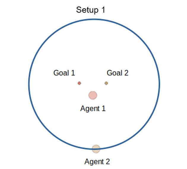
19(2) We introduce a new scenario in the multi-agent particle environment to test coexisting
qualities of agents. To be considered successful in a coexisting environment as an agent, it
needs to be able to fulfill its own task as good as possible while reducing negative impact
on others in the environment.
(3) In addition to the sum of rewards metric we use metrics from social economics to
analyze the different characteristics of the utilized policies with changed requirements in
coexisting scenarios.
3.1. Environment
Traditionally used evaluation environments have a strong bias towards strictly cooperative
solutions or are created for the purpose of cooperation. Usually only a common global goal
for all agents exists and the best behavior as defined beforehand emerges by maximizing
the sum of the joint rewards. In contrast our goal is to create an environment where
multiple goals exist that in separation do not require cooperation but interference may
happen between multiple agents when they pursue their tasks simultaneously. The closest
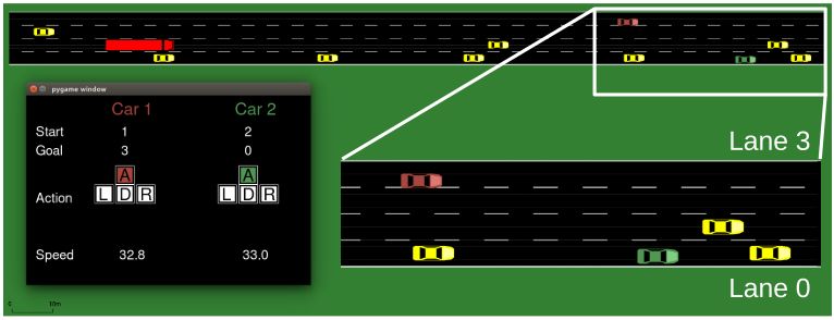
already existing scenarios are autonomous vehicle overtaking and several scenarios in
multi agent particle simulations [29] as presented by Yang et al. [60]. We build upon
the multi-agent particle environment to define our own scenarios improving the reward
design to prevent exploits regarding our research goal. To be able to show effects of our
own proposed algorithm we want the following assumptions to hold true.
• At least one agent is able to influence other agents rewards without siginificant
changes to its own reward.
• An agent should not depend on other agents to be able to reach a goal.
• An agent should not get punished if other agents take longer or do not fulfill their
respective task.
We introduce a new scenario because the first and third point are to our knowledge not
fulfilled in the other tasks we use. We did not find a multi-goal multi-agent environment
that meets all these criteria in the related work we examined. Published environments to
reproduce results are not available except for the ones of Yang et al. [60], which motivated
us to create a toy example with equally simple rules. Our toy example adds a new reward
structure to the existing environment, where one agent may exert influence over another
20agents’ reward without an effect on its own. We give a detailed description of our new
task in Chapter 4.
3.2. Evaluation
Current evaluation methods only take the sum of rewards of all agents into account. While
this is suitable for optimization for joint or global reward systems in a cooperative setting it
does not capture more intricate properties during evaluation, such as measures of fairness,
in environments, where agents have separate goals. In a system where all agents want to
independently solve their own task the global optimum of the sum might starve single
agents of reward for the greater good. While in a fully cooperative utilitaristic setting the
global maximum reward might be desired, in the real world different entities demand at
least a partial resolution of their own problem at hand even if its not the global optimum.
To further illustrate the weakness of the sum of all rewards in this scenario, consider the
simplest case of two agents Alice and Bob, each gaining a reward between zero and one.
In the first case, Alice gets a reward of one and Bob a reward of zero. In the second case,
both Alice and Bob get a reward of 0.5. If we consider the agents separately one of them
failed at his task at the benefit of the other and in case they belong to different entities,
like drivers of vehicles, the satisfaction of the found solution is low for the disadvantaged
driver. Therefore, we need a new evaluation measure of inequality for our reinforecement
learning system to asses the fairness of the reward distribution of agents. We use two
social welfare functions in conjunction to the utilitarian reward measure, the sum of
rewards. The first used metric is the Rawlsian metric [25]
RRawls = min(R1 , R2 , ..., Rn ). (3.1)
The Rawlsian metric only cares for the reward of the worst off member, by taking the
minimum reward of a member of a population. This metric tells us how well even the
worst agent is taken care of and better solutions should yield a higher minimum reward
of a member. However, this fails to account for overall better outcomes for the whole
population because we can not distinguish between the solution (1, 0) and (1, 1). Thus, it
is clear why optimizing towards such metrics is unfavorable but also that no single metric
21captures all important aspects that might be of interest.
The second metric we use is the Theil-index [53]
n (︃ )︃
1 ∑︂ ri ri
RT = ln . (3.2)
n µ µ
i=1
ri denotes the reward agent i received for an episode and µ is the mean of all rewards. If
an individual’s reward is the same as the average reward its contribution to the score is
zero and it gets higher the further away it is from the average. Thus, a better Theil-index
should score lower if we aim for a more equal distribution of rewards.
That said, both measures alone do not evaluate the fitness of a policy in isolation but
require other factors as the sum of rewards to gauge and analyze how good a policy is.
We also want to empaphize that there is no silver bullet solution in that regard and the
policy maker has to find a sweet spot in terms of this trade-off depending on the task and
desired evaluation metrics.
3.3. Multi-Goal Multi-Agent Setting
In the following section we describe the DM3 framework. We start by formulating our
multi-goal multi-agent problem formally, followed by an introduction of the mechanisms
used to construct our MARL policy gradient. To define a MARL policy gradient we define
a credit function that allows us to compute not only the credit we take towards our own
rewards, but also lets us compute the influence we have on other agents. To compute
the influence we use a concept known from psychology, the theory of mind. Instead of
estimating the influence an agent has on another agent, the agent uses a mental model to
estimate the impact of its action from the perspective of the other agent. As a consequence,
if we assume that agents share similar knowledge about the world, the agent can use the
model of itself to estimate the credit from the other agents perspective. Since we assume
a similar knowledge about the world and each agent is supposedly familiar to the same
extent on how to reach each goal, we enable parameter sharing between agents.
We present an episodic multi-goal Markov game as it is introduced by Yang et al. [60]
and adapt it to our needs. In our multi-goal MARL scenario, each agent gets a local
reward and has to maximize it for its own success. A multi-goal Markov game is a tuple
(S, On , An , P, R, G, N, γ) with |N | agents labeled by n ∈ N . In each episode, each agent
n has one fixed goal g n ∈ G that is known only to itself. At time t and global state
22st ∈ S, each agent n receives an observation ont := on (st ) ∈ On and chooses an action
ant ∈ An . The environment moves to st+1 due to joint action at := {a1t , ..., aNt }, according
to transition probability P (st+1 |st , at ). Each agent receives a reward Rtn := R(st , at , gn ),
and the learning task is to find stochastic decentralized policies π n : On × G × An →
[0, 1],
[︁∑︁conditioned on their own local observations and goals, to maximize J(π n ) :=
∞ t n
]︁
Eπ t=0 γ R(st , at , g ) ∀n ∈ N , where γ ∈ (0, 1). We start by presenting the different
techniques used.
3.3.1. Curriculum Learning and Function Augmentation
Figure 3.1.: Augmentation scheme used in the policy, value and credit network to enable
two stage learning. The observation part about oneself is seperated with ob-
servations about others. The left part only gets observations about oneself,
while the right network part that augments in stage 2 only gets information
about other agents. In the final hidden layer, before applying the activation
function, both outputs from the last intermediate hidden layers of the two
network parts are added.
Following the reasoning of Yang et al. [60] we introduce curriculum learning and a
function augmentation scheme to help alleviate the exploration problem that arises in
MARL especially with multiple goals. Exploration vs. exploitation is already a demanding
challenge in RL but the problem is further excarbated in multi-agent settings because one
23does not only need to learn how to solve an individual task, but do so in the presence
of others. To combat this issue we use the curriculum learning setup as in CM3. In the
first stage we learn a reduced single player MDP. This is reasonable as most environments
in use currently can be decomposed into a self observation part, observation of others
and observation of the environment [20]. When training for the single agent game, the
policy does only get self observations and observations of the environment. The resulting
policy is greedy w.r.t. its goal and is optimal in the single agent case. The reduction
of a multi agent MDP can be done by deleting all components of the state vector that
conveys information about other agents. As a result, in the first stage we train on the
single agent MDP and in the second stage we train with multiple agents in the multi agent
environment.
To enable the two stage learning setup we need to split the network architecture into two
separate parts as can be seen in Fig 3.1. During the first stage, the agent only observes
the environment and observations about itself, whereas in the second, information about
other agents is also observed. This seperation is achieved by decomposition of the state
space into a self observation part Oself and observation of others Oothers . During the second
stage a separate network for Oothers is introduced and the output, before applying the
activation function, of the last hidden layer hothers is added onto the last hidden layer hself
of the first network. Hence, the final layer is computed as
hout = σ(hself + hothers ), (3.3)
where σ is the nonlinear activation function of the last hidden layer. The new initialized
layers learn to process surrounding agents. By fusing the two parts the greedy initialized
networks now need to learn how to solve the task with influence of others and how to
coexist in a productive manner.
3.3.2. Credit network
To learn policies in multi-agent environments, one does not need only an estimate of how
well a state is, but actually how much each other agent contributes to his own state value.
By introducing a credit network that only computes the quality of one action towards the
goal of a single agent, we remove the necessity to observe all other agents at any given
time. Instead we only need to compute the credit of agents, that are in the vicinity and
observable from the observers point of view. The computational complexity can also be
reduced to managable levels because one does not need to take the whole state-action
24space into account. While this reduction might be insufficient for some problems this line
of reasoning is applicable, where environments and interactions are of local nature. If
an agent can be influenced by other agents outside of its view, then we would expect
learning to be severly harder. Whenever we iterate over other agents in the following
formulas m → Nt , with Nt being the number of observed agents at any given time step t,
we implicitly assume that only at that time point observable agents are taken into account
for the computation. Additionally, we fixed the amount of agents whose observation is
passed into the networks because all scenarios used only deal with local interactions.
Generalization to many more agents is not further discussed in this thesis.
Nevertheless, following the idea and proof of Yang et al. [60] we introduce a decentralized
credit assignment network Qπn (on , sm , am , gn ). The credit function evaluates how much
an agents m action am in the observed state on contributes towards goal g.
Definition: The credit function for two agents n, m is defined as
∞
[︄ ]︄
∑︂
Qπn (on , sm , am , gn ) := Eπ γ t Rtn |o0n = o, a0m = am , s0m = sm . (3.4)
t=0
Proposition: For all agents n, m, the credit function 3.4 satisfies the relations
Qn (otn , stm , atm , gn ) = E Rtn + γQn (ot+1 t+1 t+1 t t t
[︁ ]︁
n , sm , am , gn )|on = o, am = am , sm = sm
∑︂
Vn′ (otn , gn ) = πm (am |ôm , ĝ m )Qn (otn , stm , atm , gn )
am
The introduced credit function takes the current observation, the goal of an agent n, the
observed state and the action of an agent m as input. The observed state of agent m
is used as an identifier of the agent in the observation to differentiate whose action is
evaluated. This allows the assignment of a credit value to every action of each agent, even
oneself, given one’s own observation towards one’s goal. To train the credit network we
use the PPO algorithm and replace the temporal difference estimate to compute returns
with
δt = γQn (ot+1 t+1 t+1 t t t
n , sm , am , gn ) − Qn (on , sm , am , gn ), (3.5)
resulting in the credit GAE estimate Aq,t using equation 2.3.
25Sie können auch lesen