HYDROGRAPHISCHE NACHRICHTEN - Fokusthema: Numerische Modelle in der Hydrographie
←
→
Transkription von Seiteninhalten
Wenn Ihr Browser die Seite nicht korrekt rendert, bitte, lesen Sie den Inhalt der Seite unten
HYDROGRAPHISCHE
                       NACHRICHTEN
                       Journal of Applied Hydrography   02/2021   HN 118

                                                        Fokusthema:
                                                         Numerische
                                                        Modelle in der
                                                        Hydrographie
Foto: © Team Malizia
Ocean engineering
Consulting

                                               from space into depth
                                        Realise your projects in cooperation with our hydrographic services

                                                                Our hydrography engineers are happy to develop
                                                                systems tailored exactly to your needs and to
                                                                provide professional advice and support for
                                                                setting up your systems and training your staff.

                                                                MacArtney Germany benefits from being part of
                                                                the MacArtney Group and enjoys unlimited access
                                                                to cutting-edge engineering competences and
               CTDs & SVPs                                      advanced facilities.

                                                Acoustic
                                                sensors

                                                                   Software

                         Position and
                       motion sensors

                                                                   Integration

             Denmark Norway Sweden    United Kingdom France        Italy   Netherlands         Germany
                      USA   Canada   South America    Australia   Singapore        China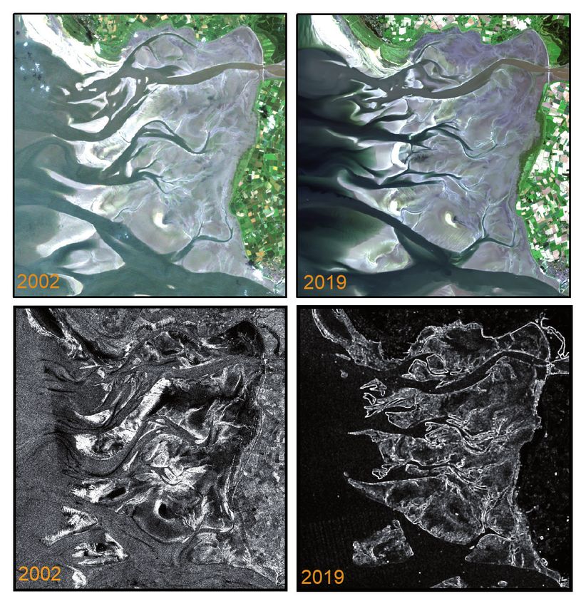
Vorwort
Liebe Leserinnen und Leser,
Fokusthema dieses Hefts sind numerische Model- Im letzten Beitrag fasst Horst Hecht die Ergeb-
le in der Hydrographie. Der Redaktion ist es jedoch nisse der 2. Generalversammlung der IHO zusam-
nur gelungen, zwei Fachbeiträge zu gewinnen, die men (Seite 48). Hecht wird von nun an in loser Fol-
sich ausführlich mit Modellierung beschäftigen. ge über die Aktivitäten der IHO berichten.
Thorger Brüning stellt mit zwei Kollegen und einer
Kollegin vom BSH das operationelle Modellsystem In dieser Ausgabe gibt es ein Novum: Zum ers-
für die Nord- und Ostsee vor (Seite 6). Caroline Ras- ten Mal hat ein Autor in einem Text für die
quin von der BAW zeigt auf, wie sich die Deutsche Hydrographischen Nachrichten ein Genderzeichen
Bucht durch den Klimawandel in Zukunft verän- verwendet. Er berichtet von einem »Team von
dern könnte (Seite 16). Im Wissenschaftsgespräch Wissenschaftler:innen, Ingenieur:innen und Tech-
mit Günther Lang – ebenfalls von der BAW – dreht niker:innen«. Das Genderzeichen steht für die-
sich auch alles um hydrodynamisch-numerische jenigen, die nicht weiblich oder männlich sind,
Lars Schiller
Modelle (Seite 20). sondern die eine nichtbinäre Geschlechtsidentität
Andere potenzielle Autorinnen und Autoren haben.
sind unserer Bitte nach einem Fachbeitrag zu nu- Die Doppelpunkte hat die Redaktion eingefügt;
merischen Modellen nicht nachgekommen. Wir im Manuskript standen Gendersternchen. Wir ha-
wissen nicht so recht, woran das liegt. An den Mo- ben uns für die typografisch zurückhaltende Aus-
delliererinnen und Modellierern? Am Thema, das zeichnung entschieden.
dann vielleicht doch eher in den Randbereich der Zwar ist das Genderzeichen in diesem Heft erst-
Hydrographie fällt? Oder schon wieder an Corona? mals abgedruckt, doch schon immer haben unse-
Erwähnung findet Modellierung auch im Bei- re Autorinnen und Autoren Ausdrücke verwendet,
trag von Stefan Marx, der davon berichtet, wie die alle mit einschließen sollen. In letzter Zeit wur-
Boris Herrmann Ozeandaten während der Vendée de oft das substantivierte Partizip oder Adjektiv
Globe gesammelt hat (Seite 44). Dieser Daten- gebraucht – wie zum Beispiel in die »Studieren-
fundus findet Eingang in neue Klimamodelle. Das den«. Doch das klappt nicht immer. Schon bei
Motto des Teams um Boris Herrmann: »A race we den »Forschenden« passt es nicht so recht, denn
must win«. Gemeint ist der Wettlauf gegen den nicht nur Forscher und Forscherinnen forschen;
von uns Menschen verursachten Klimawandel. und Forscher sind auch dann noch Forscher, wenn
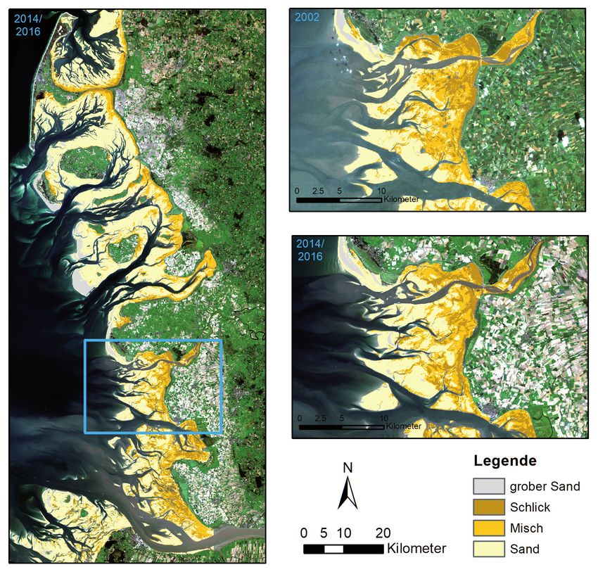
Was der Klimawandel in den letzten zwei Jahr- sie gerade nicht forschen. Auf die Idee, von den
zehnten im Schleswig-Holsteinischen Watten- »Vermessenden« zu reden, käme so schnell wohl
meer verursacht hat, zeigt die vergleichende Ana- niemand. Ich bin mir daher sicher, Sie werden den
lyse von Satellitenbilddaten, die Kerstin Stelzer mit Doppelpunkt in Zukunft häufiger mal sehen.
ihren zwei Co-Autoren für uns aufbereitet hat (Sei- Nun wünsche ich Ihnen eine anregende Lektüre
te 38). auf der Suche nach dem für Sie interessantesten
In einem weiteren Fachbeitrag bringt uns Paul Beitrag – und vielleicht auch auf der Suche nach
Wintersteller mit seinem Autorenteam die Idee den Doppelpunkten.
von NEANIAS nahe. Dabei handelt es sich um ei-
nen cloudbasierten Dienst zur Aufbereitung von
Bathymetriedaten (Seite 30).
HN 118 — 02/2021 3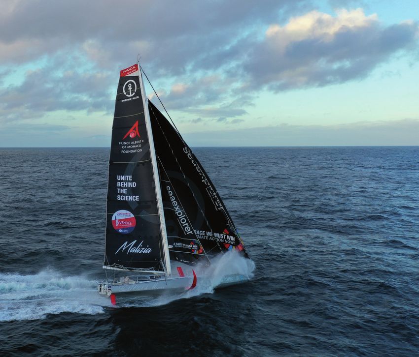
Sonic 2020                         Sonic 2022

       Sonic 2024                         Sonic 2026

     Beispiellose Leistungsfähigkeit mit 256 Beams und 1024
     Soundings bei 160° Öffnungswinkel (einstellbar) und einer Pingrate
     von 60 Hz
     Breitbandtechnologie mit Frequenzwahl in Echtzeit zwischen 200
     bis 400 kHz sowie 700 kHz optional
     Dynamisch fokussierende Beams mit einem max. Öffnungswinkel
     von 0,5° x 1° bei 400 kHz bzw. 0,3° x 0,6° bei 700 kHz
     Höchste Auflösung bei einer Bandbreite von 60 kHz, bzw. 1,25 cm
     Entfernungsauflösung
     Kombinierbar mit externen Sensoren aller gängigen Hersteller
     Flexibler Einsatz als vorausschauendes Sonar und der Fächer ist
     vertikal um bis zu 30° schwenkbar
     Zusätzliche Funktionen wie True Backscatter und Daten der
     Wassersäule
     MultiSpectral Modus™, der es den R2Sonic-Systemen ermöglicht,
     Backscatter Daten mehrerer Frequenzen in einem einzigen Durch-
     lauf zu sammeln

     Nautilus Marine Service GmbH ist der kompetente Partner in
     Deutschland für den Vertrieb von R2Sonic Fächerecholotsystemen.
     Darüber hinaus werden alle relevanten Dienstleistungen wie Instal-
     lation und Wartung kompletter hydrographischer Vermessungssys-
     teme sowie Schulung und Support für R2Sonic Kunden angeboten.
     R2Sonic ist ein amerikanischer Hersteller von modernen Fächerecho-
     loten in Breitbandtechnologie. Seit Gründung des Unternehmens
     im Jahr 2009 wurden weltweit bereits mehr als 1.500 Fächerlote
     ausgeliefert und demonstrieren so eindrucksvoll die
     außergewöhnliche Qualität und enorme Zuverlässigkeit dieser
     Vermessungssysteme.

Nautilus Marine Service GmbH · Alter Postweg 30 · D-21614 Buxtehude · Phone: +49 4161-559 03-0 · info@nautilus-gmbh.com
R2Sonic, LLC · 5307 Industrial Oaks Blvd. · Suite 120 · Austin, Texas 78735 · U.S.A. · Phone: +1-512-891-0000 · r2sales@r2sonic.com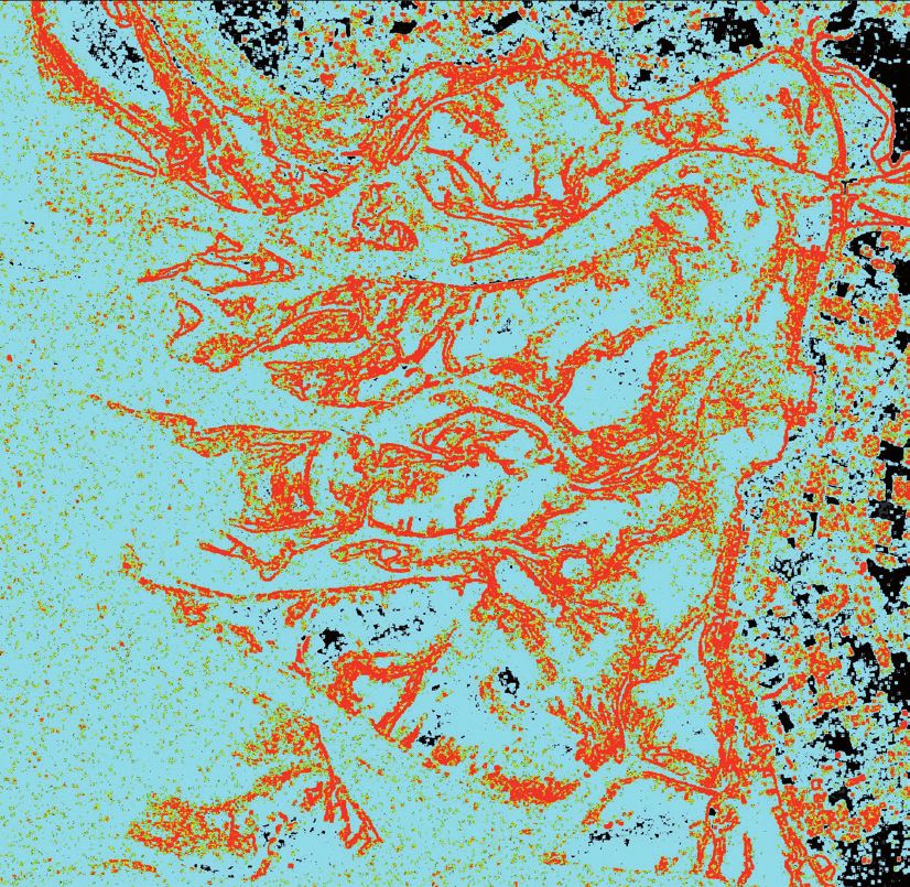
Inhaltsverzeichnis
Numerische Modelle
in der Hydrographie
Numerical modelling
6 An operational, assimilative model system for hydrodynamic and
biogeochemical applications for German coastal waters
An article by THORGER BRÜNING, XIN LI, FABIAN SCHWICHTENBERG and INA LORKOWSKI
Numerische Modellierung
16 Die Deutsche Bucht:
mögliche Zukünfte im Klimawandel
Ein Beitrag von CAROLINE RASQUIN
Wissenschaftsgespräch
20 »Das Wissen mit eigenen Worten wiedergeben«
Ein Wissenschaftsgespräch mit GÜNTHER LANG
Cloud service
30 The NEANIAS project
Bathymetric mapping and processing goes cloud
An article by PAUL WINTERSTELLER, NIKOLAOS FOSKOLOS, CHRISTIAN FERREIRA,
KONSTANTINOS KARANTZALOS, DANAI LAMPRIDOU, KALLIOPI BAIKA, JAFAR ANBAR,
JOSEP QUINTANA, STERGIOS KOKOROTSIKOS, CLAUDIO PISA and PARASKEVI NOMIKOU
Fernerkundung
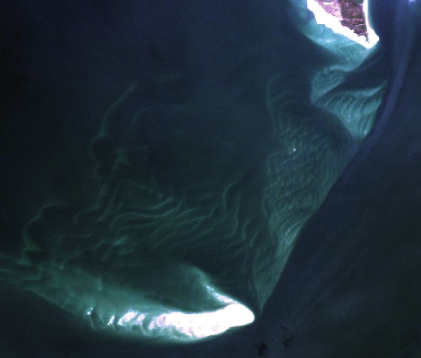
38 Den Wandel im Watt mit Satelliten im Blick
Untersuchung der Morphodynamik im Schleswig-Holsteinischen Wattenmeer durch
Satellitendatenanalyse von Prielverläufen und Sedimentklassifizierungen
Ein Beitrag von KERSTIN STELZER, MARTIN GADE und HANS-CHRISTIAN REIMERS
Open-Access-Ozeandaten
44 Der blaue Planet im Wandel
Das Klima mittels modernster Messstrategien deuten
Ein Beitrag von STEFAN MARX
Neues aus der IHO
48 Beschlüsse der 2. Generalversammlung der IHO
Ein Beitrag von HORST HECHT
Titelbild: © Team Malizia, Lorient, Juni 2020
Die nächsten Fokusthemen
HN 119 (Juni 2021) KI in der Hydrographie
HN 120 (Oktober 2021) Habitatkartierung
HN 121 (Februar 2022) Häfen und Verkehre der Zukunft
HN 118 — 02/2021 5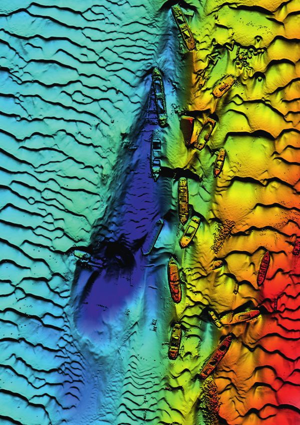
Numerical modelling                                                                                            DOI: 10.23784/HN118-01

An operational, assimilative model
system for hydrodynamic and
biogeochemical applications for
German coastal waters
An article by THORGER BRÜNING, XIN LI, FABIAN SCHWICHTENBERG and INA LORKOWSKI

The Federal Maritime and Hydrographic Agency (BSH) is introducing a new opera-
tional model system for the North and Baltic Sea, focusing on German coastal waters.
This model system newly includes a biogeochemical model and a data assimilation
component. The data streams are managed carefully to be able to conduct several
model runs per day and provide reliable forecast data for internal and external cus-
tomers. During a pre-qualification phase, model results have been validated with fo-
cus on mostly used products. Here we show validation results for tides, temperature
and oxygen. The model system is able to simulate the physical and biogeochemical
features of the North and Baltic Sea. Nevertheless, BSH is constantly developing the
model system to further improve the results and add new components to the system.

                               operational forecasting | biogeochemical modelling | hydrodynamic modelling |
                               data assimilation | North and Baltic Sea
                               operationelle Vorhersage | biogeochemische Modellierung | hydrodynamische Modellierung |
                               Datenassimilation | Nord- und Ostsee

                               Das Bundesamt für Seeschifffahrt und Hydrographie (BSH) führt ein neues operationelles Modellsystem
                               für die Nord- und Ostsee ein, dessen Schwerpunkt auf den deutschen Küstengewässern liegt. Dieses
                               Modellsystem schließt neuerdings ein biogeochemisches Modell und eine Datenassimilationskompo-
                               nente ein. Die Datenströme werden sorgfältig verwaltet, um mehrere Modellläufe pro Tag durchführen
                               zu können und zuverlässige Vorhersagedaten für interne und externe Kundinnen und Kunden zu liefern.
                               In einer Vorqualifizierungsphase wurden die Modellergebnisse validiert, wobei der Schwerpunkt auf den
                               am häufigsten verwendeten Produkten lag. Wir zeigen Validierungsergebnisse für Gezeiten, Temperatur
                               und Sauerstoff. Das Modellsystem ist in der Lage, die physikalischen und biogeochemischen Eigenschaf-
                               ten der Nord- und Ostsee zu simulieren. Nichtsdestotrotz entwickelt das BSH das Modellsystem ständig
                               weiter, um die Ergebnisse weiter zu verbessern und das System um neue Komponenten zu ergänzen.

Authors                        1 Introduction                                        is providing short-term forecasts for the most rel-
Thorger Brüning, Dr. Xin Li,   Germany is connected to the North Sea and the         evant physical parameters since the early 1990s.
Dr. Fabian Schwichtenberg      Baltic Sea. Specific physical and biogeochemical      The forecasts include information about water
and Dr. Ina Lorkowski work     processes characterise both regional seas. While      temperature and salinity, currents, water level and
at the Federal Maritime and    the North Sea has a higher salinity and is strongly   sea ice. For this purpose, BSH is operating a three-
Hydrographic Agency (BSH) in   influenced by tides, which are affecting the Ger-     dimensional baroclinic circulation model (Dick,
Hamburg.                       man coastline, the Baltic Sea has a lower salinity    Kleine and Müller-Navarra 2001; Dick, Kleine and
                               and can be partly covered by ice in winter, affect-   Janssen 2008; Brüning et al. 2014), downstream
thorger.bruening@bsh.de        ing e.g. shipping. German coastal waters and the      drift and dispersion models (Maßmann et al. 2014;
                               corresponding coastal zones are subject to many       Schmolke et al. 2020) and a two-dimensional,
                               different interests and users. This area is highly    barotropic and therefore very efficient variant of
                               impacted by ship traffic, fisheries, offshore wind    the circulation model (the storm surge model) for
                               farming, tourism and other public and economic        wind surge forecasting.
                               uses. Therefore, it is of high importance to pro-        With the increasing importance of the Marine
                               vide reliable information about the physical and      Strategy Framework Directive, the impact of eu-
                               biogeochemical status of the coastal waters. The      trophication and the development of oxygen de-
                               Federal Maritime and Hydrographic Agency (BSH)        ficiency zones in German coastal areas and in the

6                                                                                                       Hydrographische Nachrichten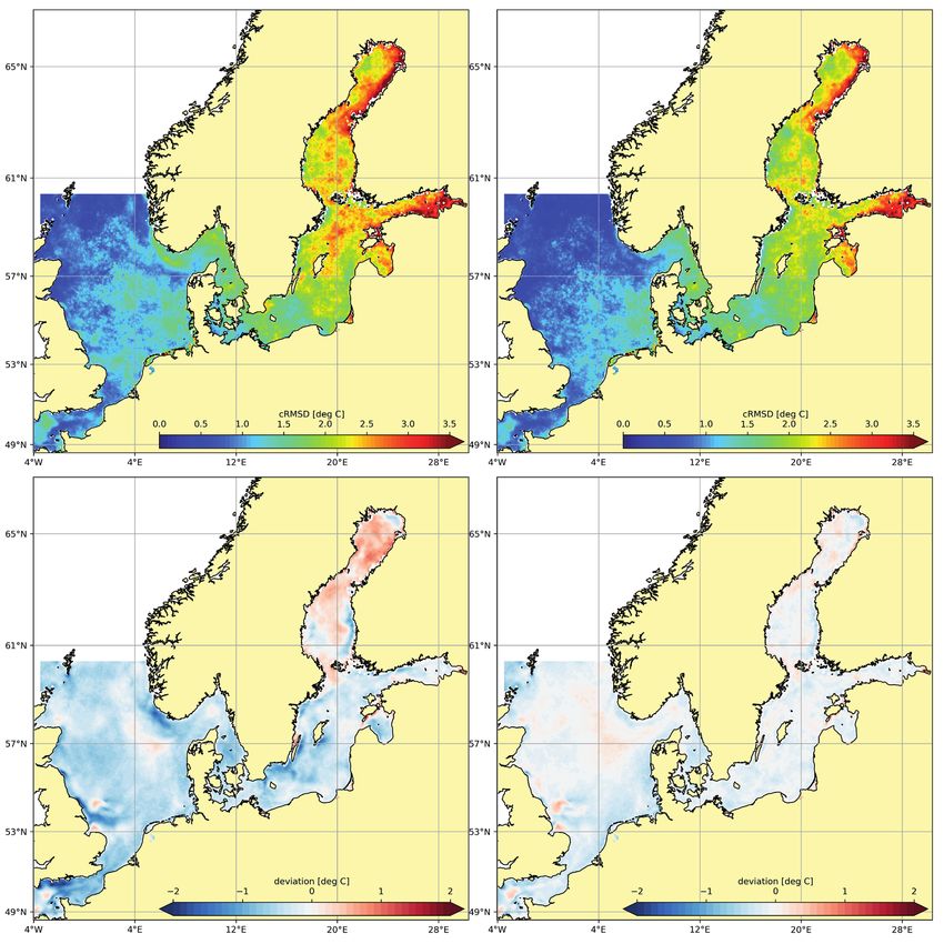
Numerical modelling

North and Baltic Sea in general (e.g. Topcu and              the concentrations of nitrogen and phosphate
Brockmann 2015; Meier et al. 2018), the need for             are taken from the Swedish Meteorological and
information about the biogeochemical status has              Hydrological Institute’s E-Hype model (Donnelly,
become more pronounced during the last years.                Andersson and Arheimer 2016; Hundecha et al.
To be able to provide short-term forecasts about             2016), delivered to BSH once per day. For the con-
important parameters of the biogeochemical en-               centrations of all other biogeochemical param-
vironment as oxygen, chlorophyll and pCO₂ con-               eters, climatological values from various sources
centration, a biogeochemical model was added to              (Pätsch and Lenhart 2008; Baltic Environment Da-
the operational model system at BSH by coupling              tabase – BED, nest.su.se/bed), but also reasonable
it to the hydrodynamic circulation model.                    constant values due to missing sources are used. If
   The physical and biogeochemical status of the             no daily updated data is available, the model runs
oceans and in particular also the German coastal             with data from the day before. Only if the supply
waters is regularly monitored by collecting in-situ          of current data is unavailable for a longer period
data and via earth observation. These data are               of time, long-term mean values of discharge and
gathered and quality controlled by organisations             climatological values of all biogeochemical con-
and services such as the Copernicus marine ser-              centrations are used.
vice (CMEMS, marine.copernicus.eu) or EmodNet                   To account for atmospheric deposition of organ-
(emodnet.eu) and are hence a valuable resource to            ic and inorganic nitrogen and organic phospho-
validate and calibrate the model system. Addition-           rus the latest available EMEP data on atmospheric
ally, assimilation of observation data can be used           deposition (emep.int) is downloaded once a year,
to further improve the quality of model results              interpolated on the model grid and recalculated to
(Kelley et al. 2002; Losa et al. 2014; Martin et al. 2015;   daily values. The atmospheric pCO₂ concentration
Nerger et al. 2016; Goodliff et al. 2019). We will pre-      is calculated based on atmospheric pCO₂ meas-
sent the first results of the new operational model          ured at Mauna Loa from the year 2017 (esrl.noaa.
framework at BSH including a biogeochemical                  gov), whereby the pCO₂ content according to esrl.
model and data assimilation.                                 noaa.gov is increased by 2 µatm every year.
                                                                Finally, two different sea surface temperature
2 The model system                                           (SST) data sets are used in the current assimilation
                                                             system: The first choice is the Advanced Very High
2.1 Data streams, forcing and setup                          Resolution Radiometer (AVHRR) SST (Kilpatrick, Po-
Four times a day, BSH is delivering an ocean fore-           destá and Evans 2001), for which a manual qual-
cast of physical and biogeochemical parameters               ity control is carried out by the BSH satellite data
to both internal and external customers. The                 service. If these data are not available or available
forecast runs start automatically at 0, 6, 12 and 18         too late for the operational procedure, the Coper-
UTC, corresponding to the analysis times of the              nicus Sentinel-3 SST (Donlon et al. 2012) is used.
atmospheric forecasts, which are provided by                 Usually, both of the satellite images are collected,
the German Weather Service (DWD) immediately                 processed and gridded by the BSH satellite data
after completion. The ocean forecasting system               service twice a day, so that the SST image is as-
requires the latest values of the parameters 10 m-           similated every 12 hours. If none of the data sets
wind, air pressure, air humidity, cloud cover and            is available in time, the forecast continues without
2 m-air temperature from the atmospheric mod-                the assimilation step.
el ICON (Zängl et al. 2015; Reinert, Frank and Prill            When all input data is available, the BSH model
2020) as meteorological input.                               system starts to calculate on two two-way nest-
  Another required input are the newest surge                ed grids. While the coarser grid covers the entire
values at the open model boundary in the north-              North Sea and Baltic Sea from ca. 4° W to ca. 30° E
ern North Sea and in the English Channel. These              and ca. 49.5° N to ca. 61° N (North Sea), respectively
are generated internally by the BSH North East At-           ca. 53° N to ca. 65.5° N (Baltic Sea) with a horizontal
lantic model (Brüning et al. 2014). In addition, tides       resolution of 3 nautical miles, the finer grid covers
based on 19 partial constituents derived from dif-           the German coastal waters from ca. 6° E to ca. 15° E
ferent measurements (e.g. Alcock and Vassie 1977;            and ca. 53° N to ca. 56.5° N with a horizontal resolu-
Cartwright, Zetler and Hamon 1979; Cartwright                tion of half a nautical mile (see Fig. 1). In the vertical
and Zetler 1985), monthly temperature and salini-            there are up to 36 layers in the coarser grid and up
ty-data from Janssen, Schrum and Backhaus (1999)             to 25 layers in the finer grid, whereas the vertical
and climatological biogeochemical data from the              resolution of both grids is identical and the higher
biogeochemical model ECOHAM (Lorkowski et al.                number of layers in the coarser grid is only due
2012) are used at the open model boundary.                   to the fact that greater water depths exists in the
  Furthermore, discharge data for the German riv-            covered area. The upper 20 m are divided in ten
ers Rhine, Elbe, Weser, Ems and Oder are obtained            layers of 2 m thickness, followed by five layers of 3
hourly via Pegelonline (pegelonline.wsv.de). The             m thickness until a water depth of 35 m and four-
discharge of the other rivers in the model area and          teen layers of 5 m thickness until a water depth of

HN 118 — 02/2021                                                                                                                           7
Numerical modelling

                                    Fig. 1: Modelled sea surface elevation on the coarser grid (left) and on the finer grid (right) on 30 June 2019 at 22:00 UTC.
                                    The tidal waves in the North Sea are clearly visible

                                   100 m. In water depths below 100 m, the resolu-                       2.2 Hydrodynamic model component
                                   tion is relatively coarse with layer thicknesses up to                The hydrodynamic core of the BSH model sys-
                                   200 m. Further details of the setup can be found in                   tem is the HIROMB-BOOS-Model (HBM) (Berg and
                                   Brüning et al. (2014) or on the BSH website (bsh.de/                  Poulsen 2012) developed by the BSH together
                                   DE/THEMEN/Modelle/modelle_node.html).                                 with European partners from the Baltic Sea region
                                      One hydrodynamic model run coupled to the                          with the configuration as described in Brüning et
                                   biogeochemical component without data assimi-                         al. (2014). HBM is a computationally very efficient
                                   lation produces a 120-hour forecast from 0 and                        ocean circulation model (Poulsen and Berg 2012a),
                                   12 UTC and a 78-hour forecast from 6 and 18 UTC.                      which was developed with a high emphasis on
                                   A second hydrodynamic model run with data as-                         portability between different computer systems.
                                   similation (without the biogeochemical compo-                         This is demonstrated by a clean code following
                                   nent) calculates a 24-hour hindcast and a 6-hour                      ANSI standards (Adams et al. 1997), which also
                                   forecast at 0 and 12 UTC.                                             allows massive parallelisation (Poulsen and Berg
                                      When the model runs are finished, numerous                         2012b; Poulsen, Berg and Raman 2014). Through a
                                   products for internal and external uses are generat-                  series of technical tests, such as the ε-tests (Brün-
                                   ed in the form of data and graphics, and the »best                    ing 2020), the technical status is checked and en-
                                   estimate« forecast is stored in the archive. Archived                 sured anew before each code release. With regard
                                   data is freely available on request by mail (opmod@                   to the physical equations, it should be noted in
                                   bsh.de). BSH provides data from the free run with-                    particular that the k-ω turbulence model (Berg
                                   out data assimilation since 2016 and results from                     2012) has been extended in recent years by sta-
                                   the simulation with data assimilation as ensemble                     bility and realisability checks. These checks are
                                   mean and standard deviation since 2021. The tem-                      necessary to ensure that the calculated current
                                   poral resolution of the archived data is listed in Ta-                data are suitable for the use of operational down-
                                   ble 1. An overview of the complex data streams is                     stream drift models for oil spill or search-and-res-
                                   displayed in Fig. 2. Hydrodynamic data from older                     cue applications, especially in extreme situations
                                   model versions are available since 2000.                              (Brüning 2020).

                            Water level    Currents        Temperature      Salinity        Sea ice concentration          Oxygen         pH              Chlorophyll
                                                                                            and thickness
 Unit                       m              m/s             °C               PSU (‰)         1 (conc.) and m (thickn.)      mmol/m³        1               mg/m³

 Temporal resolution        15 minutes     15 minutes      hourly           hourly          six-hourly                     daily (noon)   daily (noon)    daily (noon)

 Prognostic/diagnostic      diagnostic     prognostic      prognostic       prognostic      prognostic                     prognostic     diagnostic      diagnostic

 Ensemble mean and          yes            yes             yes              yes             yes                            no             no              no
 standard deviation

Table 1: Temporal resolution of the data in the BSH model archive. In addition to the deterministic data, the mean and the standard
deviation from data assimilation ensemble are also stored in the model archive for some parameters

8                                                                                                                               Hydrographische Nachrichten
Numerical modelling Fig. 2: Data streams for BSH’s operational model. Red box: required before each model run (no fall-back position). Orange boxes: required daily, with fall-back positions – both data groups are retrieved automatically. Yellow box: updated manually once a year. Green boxes: climatological data. Blue boxes: model runs/work steps at BSH 2.3 Biogeochemical model component carbon (DIC) and total alkalinity (TA) (DIC and TA For the biogeochemical model component, according to Schwichtenberg et al. (2020)). Chlo- ERGOM (Ecological ReGional Ocean Model) is ap- rophyll and Secchi depth are calculated diagnos- plied. ERGOM was originally developed for the tically (Doron et al. 2013; Neumann, Siegel and Baltic Sea (Neumann 2000). It has been adapted Gerth 2015), as well as pH and pCO₂ (Zeebe and to meet the needs for North Sea and Baltic Sea Wolf-Gladrow 2001). The sediment is not verti- as presented in Maar et al. (2011). The model con- cally resolved and consists of two nutrient state sists of 15 prognostic state variables for nutrients, variables. Fig. 3 provides an overview of the state plankton, detritus, oxygen, labile dissolved or- variables and their interaction. The HBM-ERGOM ganic nitrogen in the water column (lDON, Neu- model system has been applied in different ver- mann, Siegel and Gerth 2015), dissolved inorganic sions in a few previous studies in the North and Fig. 3: Overview of state variables and their interaction in ERGOM HN 118 — 02/2021 9
Numerical modelling

                      Baltic Sea (Maar et al. 2011; Wan et al. 2012) and has               (Pham 2001) with using the model snapshots on
                      been used in several projects at BSH (e.g. Good-                     both nested model grids of HBM (see chapter 2.1).
                      liff et al. 2019; Lorkowski and Janssen 2014) as well
                      as in the Copernicus Marine Service (Tuomi et al.                    3 Validation
                      2018) before.
                                                                                           3.1 Tides
                      2.4 PDAF                                                             BSH will provide area-wide tidal predictions for
                      With the aim of improving the forecast skill for the                 the German EEZ in the North Sea. Due to a lack
                      North and Baltic Sea, a data assimilation system                     of observational data in the open North Sea, BSH
                      has been developed at BSH within the framework                       uses model data as input for these predictions.
                      of a series of national projects (Losa et al. 2012;                  Modelled water level data of the years 2016 to
                      Losa et al. 2014; Nerger et al. 2016; Goodliff et al.                2018 were analysed with the harmonic method
                      2019). For the data assimilation component, we                       (e.g. Godín 1972). The analysis followed a two-step
                      apply the parallel data assimilation framework                       procedure with a removal of extreme water level
                      PDAF (Nerger, Hiller and Schröter 2005; Nerger and                   data and non-significant partial tides after the first
                      Hiller 2013; pdaf.awi.de), which is an open-source                   iteration. A tidal prediction for the year 2019 was
                      framework and simplifies the implementation of                       calculated and the vertices were identified. The
                      ensemble-based Kalman filtering data assimila-                       heights and times of high water (HW) and low wa-
                      tion method into a numerical model. The Local                        ter (LW) were compared with observational data
                      Error Subspace Kalman Transform Filter (LESKTF)                      at six gauges and, for better classification, with the
                      algorithm in PDAF is used in our coupled sys-                        corresponding predictions that were published
                      tem. The ESTKF is an efficient formulation of the                    in the BSH tide tables (BSH 2018). Table 2 shows a
                      Ensemble Kalman Filter (Nerger et al. 2012) that                     summary of the results.
                      has been applied in different studies to assimilate                     The predictions generated from model data
                      satellite data into different model systems (Tuomi                   show very good quality. With regard to the peak
                      et al. 2018; Androsov et al. 2019; Yang, Liu and Xu                  heights, the results are similar to those of the tide
                      2020; Li et al. 2021).                                               tables. However, the entry times of the peaks still
                         At BSH, PDAF is implemented with HBM in an                        leave room for improvement. While the mean er-
                      online mode, which calls the PDAF library directly                   rors are in the same order of magnitude as those
                      in the source code of HBM. With using the online-                    of the tide tables, the standard deviation of the
                      coupled assimilation system, the time for reading                    model-based forecast is significantly greater. In
                      input and writing output is reduced and more ef-                     particular, the standard deviation of the entry time
                      ficient for operational forecasting. Currently, the                  at gauge Fino3 is outstanding, which could be re-
                      HBM-PDAF system is the only data assimilation sys-                   lated to the relatively close position of the gauge
                      tem using online mode in the region of the Baltic                    to an amphidromic point.
                      Sea. We use an ensemble of twelve model states.
                      The state vector includes the sea surface eleva-                     3.2 Bottom oxygen saturation
                      tion, three-dimensional temperature, salinity and                    Modelled bottom oxygen saturation is compared
                      velocities. The initial physical ocean state (i.e. initial           against measurement data at three MARNET sta-
                      ensemble mean) is provided by the operational                        tions in the North and Baltic Sea (www.bsh.de/
                      HBM-run without data assimilation. The ensem-                        DE/THEMEN/Beobachtungssysteme/Messnetz-
                      ble perturbations are generated by mean of the                       MARNET/messnetz-marnet_node.html). The posi-
                      so-called second-order exact sampling method                         tion of the stations and a snapshot of the bottom

                       Tide gauge                          Tide tables                                             HBM model

                                          HW/LW heights                  HW/LW times                HW/LW heights               HW/LW times
                                        ME [m]        Std [m]      ME [min]      Std [min]        ME [m]      Std [m]       ME [min]      Std [min]

                       Borkum             0.04          0.25          –1.7          11.2           0.06         0.27           2.3             21.3

                       Cuxhaven           0.05          0.28          –0.7           8.7            0.13        0.33           15.3            14.7

                       Wittduen           0.03          0.30          –5.5           8.7           0.04          0.31         –3.9             16.3

                       Helgoland          0.03          0.25          –1.9           6.9            0.05        0.27           3.5             15.2

                       Fino1                                                                        0.03        0.22           –7.7            19.7

                       Fino3                                                                        0.11        0.25           1.2             48.6

                      Table 2: Mean error (ME) and standard deviation (Std) calculated from the predictions published in the BSH tide tables
                      and predictions based on the HBM model data for the year 2019. For the stations Fino1 and Fino3, no predictions were
                      published in the tide tables

10                                                                                                             Hydrographische Nachrichten
Numerical modelling
Fig. 4: Bottom oxygen saturation from HBM-ERGOM simulation. Snapshots for North Sea (left)
and Danish Straits and Western Baltic Sea (right). Red crosses indicate the position of monitoring stations.
(N3: Nordseeboje 3, GB: German Bight, AB: Arkona Basin)
oxygen situation in German coastal waters are dis- ficulties in reproducing SST in the Baltic Sea. In
played in Fig. 4. A seasonal oxygen minimum zone many regions of the Baltic Sea, the cRMSD is larg-
developed in the North Sea, while in the Baltic Sea er than 2.5 °C (Fig. 8). Through data assimilation,
snapshot, the permanent oxygen deficiency in the the SST forecast has significantly improved every-
Gotland and Arkona Basin and some regional sea- where in the whole model domain. In the centre
sonal minima near the coast and around Arkona of the Baltic Sea and in the Gulf of Bothnia, the
station occur. cRMSD is more obviously reduced. The bottom
At station Arkona (Fig. 5), modelled bottom oxy-
gen is principally higher than observations but the
development of the curves during the year are
comparable. Fig. 4 shows that modelled oxygen
saturation close to the station is lower, indicating
a slight spatial displacement resulting from e.g.
model bathymetry.
At the two North Sea stations (Fig. 6), bottom
oxygen saturation is also higher than observations
but the variability at both stations during the year
are well represented by the model.
In Fig. 7 modelled bottom oxygen saturation is
compared to measured values from the BSH sum-
mer cruise conducted from 27.08. to 14.09.2019.
The cruise data show an area of low oxygen,
which can be seen in the modelled data as well.
Fig. 5: Bottom oxygen saturation at station Arkona
But, as also visible in the time series plots, mod-
elled oxygen saturation is always higher than
observed, still the location of the lowest values
match quite well.
3.3 Temperature: effect of data assimilation
SST forecasting skills of both HBM free run and
HBM-PDAF runs are validated with the satellite
observations, which are used in the assimilation
processes. Fig. 8 shows the averaged validation
results over the period from July 2019 to June
2020 in the North Sea and the Baltic Sea. The
top row displays the centred root-mean-square
deviation (cRMSD) of SST forecast when no data
assimilation is applied (left) and when the data
assimilation with SST satellite is operated (right).
The comparison of SST forecasts to satellite ob-
Fig. 6: Bottom oxygen saturation at stations Nordseeboje3 and German Bight
servations shows that the HBM free run has dif-
HN 118 — 02/2021 11Numerical modelling
forecast through ensemble data assimilation is
noticed again in both the North Sea and the Bal-
tic Sea. Especially, along the Norwegian trench,
along the east coast of England and in the English
Channel, the SST bias is strongly reduced by more
than 1 °C. Through the assimilation of SST satellite
data, the yearly averaged bias is close to zero in
the whole model domain. Apparently, with SST
observational data assimilation, both model error
and bias of SST forecast have been improved.
To detect the temporal difference between the
HBM free run and HBM-PDAF run, SST is further
validated with independent in-situ observations
at the MARNET stations (positions are shown in
Fig. 4). The differences of SST between HBM free
run and HBM-PDAF run are approximately up to
Fig. 7: Comparison of bottom oxygen saturation in the German Bight. ERGOM data on the left
1.6 °C at the station Nordseeboje3 and up to 2.1 °C
are matched up in space and time with data measured during the BSH summer cruise
at the station Arkona during the compared pe-
(27.08. to 14.09.2019 with Celtic Explorer)
riod (Fig. 9). These differences change differently
with time. Large differences are displayed when
row of Fig. 8 shows the bias of forecast compared temperature rises or drops. For example, after
to the satellite observations. The improvement of the SST reaches its annual maximum in 2019, the
Fig. 8: Spatial distribution of the cRMSD (top) and bias (bottom) from the HBM free run (left)
and the HBM-PDAF run (right) in the model domain from July 2019 to June 2020
12 Hydrographische NachrichtenNumerical modelling
temperature from HBM free run drops strongly at ability and localisation of low values match quite
both stations. The SST from HBM-PDAF run is more well, making the model a useful tool to support
close to the observations and decreases slowly. It e.g. measurement campaigns or to filling gaps
shows again that the assimilation does a good job for monitoring for MSFD and other management
of eliminating biases in temperature. During the plans. However, in all cases shown, the saturation
winter and spring, on the other hand, the tem- is higher than observed values. Furthermore, the
peratures from HBM free run and HBM-PDAF run stratification in the model is sometimes too weak
at these two stations are generally quite close to (not shown). This affects biogeochemical and
each other (Fig. 9). One of the reasons might be physical fields alike.
due to the lack of satellite observations. In order to improve the forecast capability of the
model in general, we will massively expand the as-
4 Discussion and next steps similation of observational data. For example, as
With the presented operational system, BSH is able requested by customers, the data assimilation of
to provide reliable daily forecast data to external sea ice parameters will be implemented in 2021.
and internal users. The model system uses state- Furthermore, the addition of temperature and sa-
of-the-art techniques to simulate the main physical linity profiles into the assimilation system should
and biogeochemical features of German coastal improve stratification, especially in the Baltic Sea, Acknowledgements
waters. The addition of a biogeochemical model to which should also lead to an improvement of We would like to thank
the modelling framework widens the range of data biogeochemical model results in deeper model Andreas Boesch from the
products for different purposes. The inclusion of layers (e.g. bottom oxygen). A future step would BSH Tidal Service for the
data assimilation improves the quality of simulated then be the direct assimilation of biogeochemical preparation of the harmonic
SST. Currently the free run and the run with data as- data to further improve this model component. analyses, the calculation of
similation are running in parallel but in the very near Additionally, a new setup with a higher horizon- the tidal prediction quality, as
future, the hydrodynamic restart file of the forecast tal and vertical grid resolution based on an ac- well as his kind suggestions
with data assimilation should be used for the next tual, high-resolution bathymetry data set is being and comments regarding this
forecast run of the model with biogeochemical planned. In this setup, the model area will also publication.
component with the aim of further improving the include large parts of the North-East Atlantic. By We would also like to thank
forecast skill of the model system. moving the open model boundary from the shelf Annika Grage, Larissa Müller
Nevertheless, there are also weaknesses of the to deep-water areas of the North Atlantic, high- and Kevin Hett for providing
current system, which we aim to improve in the quality data from global tide models can be used in-situ data.
future. As shown, the tides are represented well in as forcing at the open boundaries. This will hope-
terms of water level, but the timing of the peaks fully lead to significant improvements in the repre-
should become more accurate. For modelled sentation of tides in the North Sea and especially
oxygen saturation, on the other hand, the vari- in the German Bight. //
Fig. 9: Comparison of time series of surface temperature from the HBM free run and HBM-PDAF run
with in-situ data at station Nordseeboje3 (top) and station Arkona (bottom)
HN 118 — 02/2021 13Numerical modelling
References
Adams, Jeanne C.; Walter S. Brainerd et al. (1997): Fortran 95 assimilation. Ocean Dynamics, DOI: 10.1007/s10236-019-
handbook: complete ISO/ANSI reference. MIT press 01299-7
Alcock, GA; JM Vassie (1977): Offshore Tide Gauge Data- Hundecha, Yeshewatesfa; Berit Arheimer et al. (2016): A
Northern North Sea (JONSDAP 76). Data Report No. 10, regional parameter estimation scheme for a pan-European
Bidston Observatory, Birkenhead multi-basin model. Journal of Hydrology: Regional Studies,
Androsov, Alexey; Lars Nerger et al. (2019): On the assimilation DOI: 10.1016/j.ejrh.2016.04.002
of absolute geodetic dynamic topography in a global Janssen, Frank; Corinna Schrum; J. O. Backhaus (1999): A
ocean model: impact on the deep ocean state. Journal of climatological data set of temperature and salinity for the
Geodesy, DOI: 10.1007/s00190-018-1151-1 Baltic Sea and the North Sea. Deutsche Hydrographische
Berg, Per (2012): Mixing in HBM. Scientific Report, Danish Zeitschrift, DOI: 10.1007/BF02933676
Meteorological Institute, Copenhagen Kelley, John G. W.; David W. Behringer et al. (2002): Assimilation
Berg, Per; Jacob Weismann Poulsen (2012): Implementation of SST Data into a Real-Time Coastal Ocean Forecast
details for HBM. Technical Report 12-11, Danish System for the U.S. East Coast. Weather and Forecasting,
Meteorological Institute, Copenhagen DOI: 10.1175/1520-0434(2002)0172.0.CO;2
Brüning, Thorger (2020): Improvements in turbulence model Kilpatrick, K. A.; G. P. Podestá; R. Evans (2001): Overview of the
realizability for enhanced stability of ocean forecast and NOAA/NASA advanced very high resolution radiometer
its importance for downstream components. Ocean Pathfinder algorithm for sea surface temperature and
Dynamics, DOI: 10.1007/s10236-020-01353-9 associated matchup database. Journal of Geophysical
Brüning, Thorger; Frank Janssen et al. (2014): Operational Research: Oceans, DOI: 10.1029/1999JC000065
Ocean Forecasting for German Coastal Waters. Die Küste, Li, Zhijie; Zhaoyi Wang et al. (2021): Evaluation of global
Nr. 81, S. 273–290 high-resolution reanalysis products based on the
BSH (2018): Gezeitentafeln 2019: Europäische Gewässer. Chinese Global Oceanography Forecasting System.
Bundesamt für Seeschifffahrt, ISSN: 0084-9774 Atmospheric and Oceanic Science Letters. DOI: 10.1016/j.
Cartwright, D. E.; B. D. Zetler (1985): Pelagic tidal constants 2. aosl.2021.100032
IAPSO Publication Scientifique, No. 33 Lorkowski, Ina; Johannes Pätsch et al. (2012): Interannual
Cartwright, D.E.; B. D. Zetler; B. V. Hamon (1979): Pelagic tidal variability of carbon fluxes in the North Sea (1970–2006)
constants; IAPSO Publication Scientifique, No. 30 – Abiotic and biotic drivers of the gas-exchange of
Dick, Stephan; Eckhard Kleine; Frank Janssen (2008): A New CO₂. Estuarine, Coastal and Shelf Science, DOI: 10.1016/j.
Operational Circulation Model for the North Sea and the ecss.2011.11.037
Baltic Using a Novel Vertical Co-ordinate – Setup and Lorkowski, Ina; Frank Janssen (2014): Modelling the
First Results. In: H. Dalhin; M. J. Bell et al. (Editors): Coastal biogeochemical and physical state of the North and Baltic
to Global Operational Oceanography: Achievements Seas. Proceedings of the Seventh EuroGOOS International
and Challenges. Proceedings of the Fifth International Conference, pp. 299–306
Conference on EuroGOOS, 20–22 May 2008, Exeter, Losa, Svetlana N.; Sergey Danilov et al. (2014): Assimilating
pp. 225–231 NOAA SST data into the BSH operational circulation model
Dick, Stephan; Eckhard Kleine; Sylvin H. Müller-Navarra for the North and Baltic Seas: Part 2. Sensitivity of the
(2001): The operational circulation model of BSH (BSH forecast’s skill to the prior model error statistics. Journal of
cmod). Model description and validation. Berichte des Marine Systems, DOI: 10.1016/j.jmarsys.2013.06.011
Bundesamtes für Seeschifffahrt und Hydrographie. Losa, Svetlana N.; Jens Schröter et al. (2012): Assimilating NOAA
29/2001, 48. Hamburg SST data into the BSH operational circulation model for the
Donlon, Craig; Bruno Berruti et al. (2012): The Global North and Baltic Seas: Inference about the data. Journal of
Monitoring for Environment and Security (GMES) Marine Systems, DOI: 10.1016/j.jmarsys.2012.07.008
Sentinel-3 mission. Remote Sensing of Environment, Maar, Marie; Eva Friis Møller et al. (2011): Ecosystem
DOI: 10.1016/j.rse.2011.07.024 modelling across a salinity gradient from the North Sea
Donnelly, Chantal; Jafet C. M. Andersson; Berit Arheimer. to the Baltic Sea. Ecological Modelling, DOI: 10.1016/j.
(2016): Using flow signatures and catchment ecolmodel.2011.03.006
similarities to evaluate the E-HYPE multi-basin Martin, Matthew J.; M. Balmaseda et al. (2015): Status
model across Europe. Hydrological Sciences Journal, and future of data assimilation in operational
DOI: 10.1080/02626667.2015.1027710 oceanography. Journal of Operational Oceanography,
Doron, Maéva; Pierre Brasseur et al. (2013): Stochastic DOI: 10.1080/1755876X.2015.1022055
estimation of biogeochemical parameters from Globcolour Maßmann, Silvia; Frank Janssen et al. (2014): An operational
ocean colour satellite data in a North Atlantic 3D ocean oil drift forecasting system for German coastal waters. Die
coupled physical–biogeochemical model. Journal of Küste, Nr. 81, pp. 255-271
Marine Systems, DOI: 10.1016/j.jmarsys.2013.02.007 Meier, H. E. Markus; Germo Väli et al. (2018): Recently
Godín, Gabriel (1972): The Analysis of Tides. University of accelerated oxygen consumption rates amplify
Toronto Press, Ontario deoxygenation in the Baltic Sea. Journal of Geophysical
Goodliff, Michael; Thorger Bruening et al. (2019): Temperature Research: Oceans, DOI: 10.1029/2017JC013686
assimilation into a coastal ocean-biogeochemical Nerger, Lars; Wolfgang Hiller (2013): Software for Ensemble-
model: assessment of weakly and strongly coupled data based Data Assimilation Systems – Implementation
14 Hydrographische NachrichtenNumerical modelling
Strategies and Scalability. Computers and Geosciences, Poulsen, Jacob Weismann; Per Berg; Karthik Raman (2014):
DOI: 10.1016/j.cageo.2012.03.026 Better Concurrency and SIMD On The HIROMB-BOOS-
Nerger, Lars; Wolfgang Hiller; Jens Schröter (2005): PDAF – MODEL (HBM) 3D Ocean Code. In: James Jeffers; Jim
The Parallel Data Assimilation Framework: Experiences Reinders (Eds.): High Performance Parallelism Pearls:
with Kalman Filtering. 11th ECMWF Workshop on Use Multicore and Many-core Programming Approaches.
of High Performance Computing in Meteorology, DOI: Morgan Kaufmann Publishing
10.1142/9789812701831_0006 Reinert, Daniel; Helmut Frank; Florian Prill (2020): ICON
Nerger, Lars; Tijana Janjic et al. (2012): A unification of database reference manual, Version 2.2.1. DWD
ensemble square root Kalman filters. Monthly Weather Schmolke, Stefan; Katrin Ewert et al. (2020): Environmental
Review, DOI: 10.1175/MWR-D-11-00102.1 Protection in Maritime Traffic – Scrubber Wash Water
Nerger, Lars; Svetlana N. Losa et al. (2016): The HBM-PDAF Survey. Umweltbundesamt
assimilation system for operational forecasts in the North Schwichtenberg, Fabian; Johannes Pätsch et al. (2020): The
and Baltic Seas. Operational Oceanography for Sustainable impact of intertidal areas on the carbonate system of the
Blue Growth. Proceedings of the Seventh EuroGOOS southern North Sea. Biogeosciences, DOI: 10.5194/bg-17-
International Conference, 28–30 October 2014, Lisbon 4223-2020
Neumann, Thomas (2000): Towards a 3D-ecosystem model Topcu, H. Dilek; Uwe H. Brockmann (2015): Seasonal oxygen
of the Baltic Sea. Journal of Marine Systems, DOI: 10.1016/ depletion in the North Sea, a review. Marine Pollution
S0924-7963(00)00030-0 Bulletin, DOI: 10.1016/j.marpolbul.2015.06.021
Neumann, Thomas; Herbert Siegel; Monika Gerth (2015): Tuomi, Laura; Jun She et al. (2018): Overview of CMEMS BAL
A new radiation model for Baltic Sea ecosystem MFC Service and Developments. Proceedings of the Eigth
modelling. Journal of Marine Systems, DOI: 10.1016/j. EuroGOOS International Conference, 3–5 October 2017,
jmarsys.2015.08.001 Bergen, pp. 261–268
Pätsch, Johannes; Herman-J. Lenhart (2008): Daily Loads of Wan, Zhenwen; Jun She et al. (2012): Assessment of a physical-
Nutrients, Total Alkalinity, Dissolved Inorganic carbon and biogeochemical coupled model system for operational
Dissolved organic carbon of the European Continental service in the Baltic Sea. Ocean Science, DOI. 10.5194/os-8-
Rivers of the Years 1977–2006. Berichte aus dem Zentrum 683-2012
für Meeres- und Klimaforschung, Uni Hamburg Yang, Chao-Yuan; Jiping Liu; Shiming Xu (2020): Seasonal
Pham, Dinh Tuan (2001): Stochastic methods for sequential Arctic Sea Ice Prediction Using a Newly Developed Fully
data assimilation in strongly nonlinear systems. Monthly Coupled Regional Model With the Assimilation of Satellite
Weather Review, DOI: 10.1175/1520-0493(2001)1292.0.CO;2 Earth Systems, DOI: 10.1029/2019MS001938
Poulsen, Jacob Weismann; Per Berg (2012a): More details on Zängl, Günther; Daniel Reinert et al. (2015): The ICON
HBM – general modelling theory and survey of recent (ICOsahedral Non-hydrostatic) modelling framework
studies. Technical Report 12-16, Danish Meteorological of DWD and MPI-M: Description of the non-hydrostatic
Institute, Copenhagen dynamical core. Quarterly Journal of the Royal
Poulsen, Jacob Weismann; Per Berg (2012b): Thread scaling Meteorological Society, DOI: 10.1002/qj.2378
with HBM. Technical Report 12-20. Danish Meteorological Zeebe, Richard E.; Dieter Wolf-Gladrow (2001): CO₂ in seawater:
Institute, Copenhagen equilibrium, kinetics, isotopes. Gulf Professional Publishing
Hydrographische Nachrichten Chefredakteur:
HN 118 – Februar 2021 Lars Schiller
E-Mail: lars.schiller@dhyg.de
Journal of Applied Hydrography
Redaktion:
Offizielles Organ der Deutschen Hydrographischen Peter Dugge, Dipl.-Ing.
Gesellschaft – DHyG Horst Hecht, Dipl.-Met.
Holger Klindt, Dipl.-Phys.
Herausgeber: Dr. Jens Schneider von Deimling
Deutsche Hydrographische Gesellschaft e. V. Stefan Steinmetz, Dipl.-Ing.
c/o Innomar Technologie GmbH Dr. Patrick Westfeld
Schutower Ringstraße 4
18069 Rostock Hinweise für Autoren und Inserenten:
www.dhyg.de > Hydrographische Nachrichten >
ISSN: 1866-9204 © 2021 Mediadaten und Hinweise
HN 118 — 02/2021 15Numerische Modellierung DOI: 10.23784/HN118-02
Die Deutsche Bucht:
mögliche Zukünfte im Klimawandel
Ein Beitrag von CAROLINE RASQUIN
Meeresspiegel, Meteorologie, Topographie des Wattenmeers, binnenseitiger Abfluss
in die Ästuare: All dies wird durch den Klimawandel beeinflusst. Und das nicht einzeln
nacheinander, sondern alles parallel auf unterschiedlichen Zeitskalen, weil alles mit
allem zusammenhängt. Wir wagen einen Blick in die Zukunft und zeigen mit Hilfe von
numerischen Modellen, was uns in der Deutschen Bucht erwarten könnte.
numerische Modellierung | Klimawandel | Meeresspiegelanstieg | Wattenmeerentwicklung | Deutsche Bucht
numerical modelling | climate change | sea level rise | tidal flat development | German Bight
Sea level, meteorology, topography of the Wadden Sea, inland runoff into the estuaries: all these are influ-
enced by climate change. And not one after the other, but all in parallel on different time scales, because
everything is connected to everything else. We dare to look into the future and, with the help of numeri-
cal models, show what could await us in the German Bight.
Autorin Im BMVI-Expertennetzwerk arbeiten seit 2016 sie- biete der Deutschen Bucht beinhalten. Im Gegen-
Caroline Rasquin ist wissen- ben Ressortforschungseinrichtungen und Fachbe- satz zu klassischen Wenn-Dann-Studien, bei de-
schaftliche Mitarbeiterin bei hörden des Bundesministeriums für Verkehr und nen zwischen Szenarien immer nur ein Parameter,
der BAW in Hamburg. digitale Infrastruktur (BMVI) verkehrsträgerüber- wie z. B. der Meeresspiegel, variiert wird, werden
greifend zusammen, um durch Klimaverände- bei dieser Vorgehensweise mehrere Parameter auf
caroline.rasquin@baw.de rungen und extreme Wetterereignisse bedingte einmal geändert. Das führt dazu, dass keine ein-
Betroffenheiten für Verkehr und Infrastruktur zu deutigen Rückschlüsse gezogen werden können,
bestimmen und beispielhaft Anpassungsoptio- welches Änderungssignal von welchem Parame-
nen zu entwickeln. Schwerpunkte der BAW (Bun- ter stammt. Die Änderungen liefern aber Hinweise
desanstalt für Wasserbau) liegen unter anderem über die Größenordnung möglicher zukünftiger
auf der Fragestellung, welche Änderungen von Entwicklungen. Auf diese Weise können kritische
Hydrodynamik und Sedimenttransport in den Punkte erkannt und bei Bedarf mögliche Anpas-
Küstenbereichen der Deutschen Bucht bei einem sungsmaßnahmen entwickelt werden. Die Infor-
Meeresspiegelanstieg zu erwarten sind und wel- mationen und Daten für die jeweiligen Szenarien-
che Folgen sich daraus für den Verkehrsträger Pakete wurden durch die Bundesbehörden BSH
Wasserstraße ergeben. Die im BMVI-Experten- (Bundesamt für Seeschifffahrt und Hydrographie),
netzwerk entwickelten Methoden und Verfahren DWD (Deutscher Wetterdienst), BfG (Bundesan-
sollen im DAS-Basisdienst »Klima und Wasser« der stalt für Gewässerkunde) und BAW zusammen er-
Deutschen Anpassungsstrategie in den Routine- arbeitet (Schade et al. 2020; BAW 2020a).
betrieb überführt werden. Untersucht werden charakteristische Jahre der
In vorangegangenen Studien, z. B. KLIWAS (BAW Zeitscheiben »Referenz« (1971 bis 2000), »nahe Zu-
2015), ProWaS (BAW 2018), wurden bereits zahlrei- kunft« (2031 bis 2060) und »ferne Zukunft« (2071
che an der Küste vom Klimawandel beeinflusste bis 2100). Als Klimaszenario wird das »Weiter-wie-
Komponenten (Meeresspiegelanstieg, Abfluss aus bisher«-Szenario RCP8.5 verwendet. Die charakte-
den Flüssen, Meteorologie) einzeln untersucht. Im ristischen Jahre sollen möglichst typische Verhält-
BMVI-Expertennetzwerk kombinieren wir die ein- nisse der jeweiligen Zeitscheibe abbilden.
zelnen Sensitivitätsstudien und untersuchen, wie Für die Untersuchungen wird ein hydrodyna-
eine mögliche Zukunft aussehen kann, in der die misch-numerisches Modell verwendet. Das Mo-
zu erwartenden Veränderungen zusammenspie- dell basiert auf dem hydrodynamisch-numeri-
len. schen Verfahren UnTRIM² (Casulli 2008; Casulli und
Dafür werden unterschiedliche Szenarien-Pake- Stelling 2011), das die dreidimensionalen Flachwas-
te geschnürt, die jeweils mögliche und plausible sergleichungen und die dreidimensionale Trans-
zu erwartende Verhältnisse hinsichtlich des Wind- portgleichung für Salz, Schwebstoffe und Wärme
klimas, des binnenseitigen Abflusses in die Ästua- auf einem orthogonalen, unstrukturierten Gitter
re, des Meeresspiegelanstiegs, des Salzgehalts in löst (Casulli und Walters 2000).
der Nordsee sowie der Topographie der Wattge- Das Modellgebiet umfasst die gesamte Deut-
16 Hydrographische NachrichtenNumerische Modellierung
sche Bucht von den Niederlanden bis Dänemark
sowie die angrenzenden Ästuare von Elbe, Weser
und Ems mit den jeweiligen Nebenflüssen (Abb. 1).
Die Auflösung des Rechengitters ist räumlich va-
riabel mit einer Kantenlänge von 5 km am offenen
Seerand, 300 m im Küstenvorfeld und etwa 50 m
in den Ästuaren. Die verwendete Subgrid-Tech-
nologie ermöglicht in den küstennahen Bereichen
und in den Ästuaren eine detailliertere Darstellung
der Topographie (Sehili et al. 2014). In den hoch
aufgelösten Bereichen (z. B. dem Dollart, auf den
Watten oder der Elbmündung) liegt auf Subgrid-
Ebene eine Auflösung von etwa 10 bis 20 m vor.
Aufgrund der hohen Auflösung kann das Über-
fluten und Trockenfallen in der intertidalen Zone
gut reproduziert werden. Die hohe Auflösung des
Modells im küstennahen Bereich ist besonders bei
der Untersuchung von Meeresspiegelanstiegen
entscheidend (Rasquin et al. 2020).
Szenarien der Untersuchung
Abb. 1: Gebiet des Deutsche-Bucht-Modells der BAW (nach Rasquin et al. 2020)
Zur Steuerung des Deutsche-Bucht-Modells wer-
den Randdaten für den Wind, die binnenseitigen
Abflüsse, den Meeresspiegelanstieg, den Salzge- oder auch der Küstenlängstransport sowie der
halt in der Nordsee sowie die Topographie der Eintrag aus den Ästuaren. Ein Aufwachsen der
Wattgebiete benötigt. Diese Parameter werden Wattflächen kann den Auswirkungen eines Mee-
zu einzelnen Szenarien-Paketen kombiniert. Die resspiegelanstiegs auf die Tidedynamik teilweise
Randdaten für Wind, Abfluss und Salzgehalt stam- entgegenwirken (Wachler et al. 2020). Aufbauend
men aus gekoppelten Klimasimulationen und sind auf diesen Erkenntnissen werden für jeden ange-
somit in sich konsistent. nommenen Meeresspiegelanstieg Topographie-
Für den Meeresspiegel ist zukünftig mit einem szenarien entwickelt. Diese weisen einem Sze-
beschleunigten Anstieg zu rechnen (IPCC 2014, nario eine bestimmte Erhöhung der Watten zu.
2019). Die Bandbreite der möglichen Anstiegsra- Es wird hier vorausgesetzt, dass diese Erhöhung
ten ist groß. Basierend auf dem RCP8.5-Szenario geringer ausfällt als der dem Szenario zugehörige
wird exemplarisch im Szenario-Paket »Nahe Zu- Meeresspiegelanstieg. Die Rinnen im Wattgebiet
kunft« ein Meeresspiegelanstieg von 0,30 m und werden vertieft, da angenommen wird, dass etwa
im Szenario-Paket »Ferne Zukunft« ein Anstieg von 30 bis 40 % des zur Watterhöhung benötigten Ma-
0,80 m angenommen. Zusätzlich wird auch ein terials aus den Rinnen stammt. Die Vertiefung der
High-End-Szenario mit einem Anstieg um 1,74 m Rinnen wird prozentual vorgenommen. So wird er-
untersucht. reicht, dass tiefe Abschnitte stärker vertieft werden
Bei einem Anstieg des Meeresspiegels wird als flachere Übergänge zu den Wattflächen.
nicht nur die Tidedynamik beeinflusst, sondern Die hier getroffenen Annahmen werden verein-
auch die Topographie im Küstenbereich, da diese fachend für das gesamte Wattenmeer getroffen.
ein morphodynamisches Gleichgewicht mit den Es ist jedoch zu beachten, dass sich die morpholo-
hydrodynamischen Kräften anstrebt (Friedrichs gischen Reaktionen lokal sehr unterschiedlich aus-
2011). Die Wattflächen können bis zu einem gewis- prägen können. Zudem zeigen die Wasserstände
sen Grad des Meeresspiegelanstiegs mitwachsen in der Elbe eine unterschiedliche Reaktion je nach-
(z. B. Becherer et al. 2018). Dies kann jedoch nur ge- dem, ob auch die Watten im Ästuar angehoben
schehen, wenn eine ausreichende Sedimentver- werden (BAW 2020b).
fügbarkeit gegeben ist. Sedimentquellen sind zum Die untersuchten Szenarien sind in Tabelle 1 auf-
Beispiel die Wattrinnen, Sandbänke, Barriereinseln geführt.
Szenarienkürzel REF NZ30 FZ80 FZ174
Zeitscheibe bzw. Szenario Referenz Nahe Zukunft Ferne Zukunft Ferne Zukunft
Verwendeter Meeresspiegelanstieg 0m 0,30 m 0,80 m 1,74 m
Verwendetes Topographieszenario Keine Änderung Watten um 0,20 m Watten um 0,50 m Watten um 0,65 m
erhöht, Rinnen um erhöht, Rinnen um erhöht, Rinnen um
4 % vertieft 11 % vertieft 14 % vertieft
Tabelle 1: Untersuchte Szenarien mit verwendeten Meeresspiegelanstiegen und Topographieszenarien
HN 118 — 02/2021 17Numerische Modellierung
Analyse und Ergebnisse dargestellt. Es ist jeweils der Referenzzustand
Für jedes der Szenarien-Pakete wird ein hydrologi- (kein Meeresspiegelanstieg und keine topogra-
sches Jahr (1. November bis 31. Oktober) mit dem phischen Veränderungen) gezeigt sowie das Sze-
Deutsche-Bucht-Modell simuliert. Die Ergebnisse nario FZ80 (siehe Tabelle 1). Eine Erhöhung der
können je nach Forschungsfrage auf verschiedene Wasserstände kann vielerlei Auswirkungen haben.
Arten analysiert werden. Es können sowohl tide- An der Küste Norddeutschlands und in den Ästua-
abhängige als auch tideunabhängige Kennwer- ren wird das Hinterland über Siele entwässert, was
te erstellt werden (BAWiki 2021). Dabei kann der größtenteils im Freispiegelgefälle erfolgt. Steigen
Analysezeitraum das gesamte hydrologische Jahr, die Außenwasserstände durch den Klimawandel
einzelne Spring-Nipp-Zyklen oder auch einzelne deutlich an, wird das Entwässerungsfenster (der
Ereignisse umfassen. Zeitraum, in dem der Wasserstand vor dem Deich
Bei der Interpretation der Ergebnisse muss stets niedriger ist als im Siel hinter dem Deich) deutlich
bedacht werden, dass es sich um Szenarien han- kleiner. Im Extremfall muss mit Pumpen entwäs-
delt und die Ergebnisse keine Prognosen für ein sert werden. Auch können erhöhte Wasserstände
bestimmtes zukünftiges Jahr darstellen. Die Mo- eine Herausforderung für den Küstenschutz dar-
dellsimulationen liefern unter den angenomme- stellen.
nen Randbedingungen belastbare Aussagen und Durch einen Anstieg des Meeresspiegels än-
können somit Anhaltspunkte zu möglichen Ent- dern sich nicht nur die Wasserstände, sondern die
wicklungen geben. Die Ergebnisse sind in einem Tidedynamik insgesamt. Zum Beispiel wird auch
Bildatlas veröffentlicht (BAW 2020a). An dieser Stel- das Verhältnis zwischen Flut- und Ebbestrom-
le sollen einige ausgewählte Ergebnisse vorgestellt geschwindigkeit beeinflusst. Eine damit verbun-
werden. dene Auswirkung kann ein erhöhter Eintrag von
Durch einen Anstieg des Meeresspiegels wer- Feinsedimenten in die Ästuare sein. Falls sich die
den sich Tidehoch- und Tideniedrigwasser erhö- Wassertiefe aufgrund eines erhöhten Sediment-
hen. Diese Entwicklung ist in Abb. 2 und Abb. 3 imports stärker verringert als sie sich durch den
Abb. 2: Mittleres Tideniedrigwasser für die Szenarien REF und FZ80 (siehe Tabelle 1)
Abb. 3: Mittleres Tidehochwasser für die Szenarien REF und FZ80 (siehe Tabelle 1)
18 Hydrographische NachrichtenSie können auch lesen


