Internationale Mathematische Nachrichten International Mathematical News Nouvelles Mathématiques Internationales
←
→
Transkription von Seiteninhalten
Wenn Ihr Browser die Seite nicht korrekt rendert, bitte, lesen Sie den Inhalt der Seite unten
Internationale Mathematische Nachrichten
International Mathematical News
Nouvelles Mathématiques Internationales

Die IMN wurden 1947 von R. Inzin-             reichischen Mathematischen Gesellschaft
ger als „Nachrichten der Mathematischen       bezogen.
Gesellschaft in Wien“ gegründet. 1952         Jahresbeitrag: 35,–
wurde die Zeitschrift in „Internationale
                                              Bankverbindung:
Mathematische Nachrichten“ umbenannt
                                              IBAN AT83-1200-0229-1038-9200 bei
und war bis 1971 offizielles Publikati-
                                              der Bank Austria-Creditanstalt (BIC-Code
onsorgan der „Internationalen Mathema-
                                              BKAUATWW ).
tischen Union“.
Von 1953 bis 1977 betreute W. Wunder-
lich, der bereits seit der Gründung als Re-
dakteur mitwirkte, als Herausgeber die
IMN. Die weiteren Herausgeber waren
H. Vogler (1978–79), U. Dieter (1980–
81, 1984–85), L. Reich (1982–83), P. Flor
(1986–99), M. Drmota (2000–2007) und
J. Wallner (2008–2017).

Herausgeber:
Österreichische Mathematische Gesell-
schaft, Wiedner Hauptstraße 8–10/104,
A-1040 Wien. email imn@oemg.ac.at,
http://www.oemg.ac.at/

Redaktion:
C. Fuchs (Univ. Salzburg, Herausgeber)        Eigentümer, Herausgeber und Verleger:
H. Humenberger (Univ. Wien)                   Österr. Math. Gesellschaft. Satz: Österr.
R. Tichy (TU Graz)                            Math. Gesellschaft. Druck: Weinitzen-
J. Wallner (TU Graz)                          druck, 8044 Weinitzen.

Bezug:                                         c 2021 Österreichische Mathematische
Die IMN erscheinen dreimal jährlich und       Gesellschaft, Wien.
werden von den Mitgliedern der Öster-         ISSN 0020-7926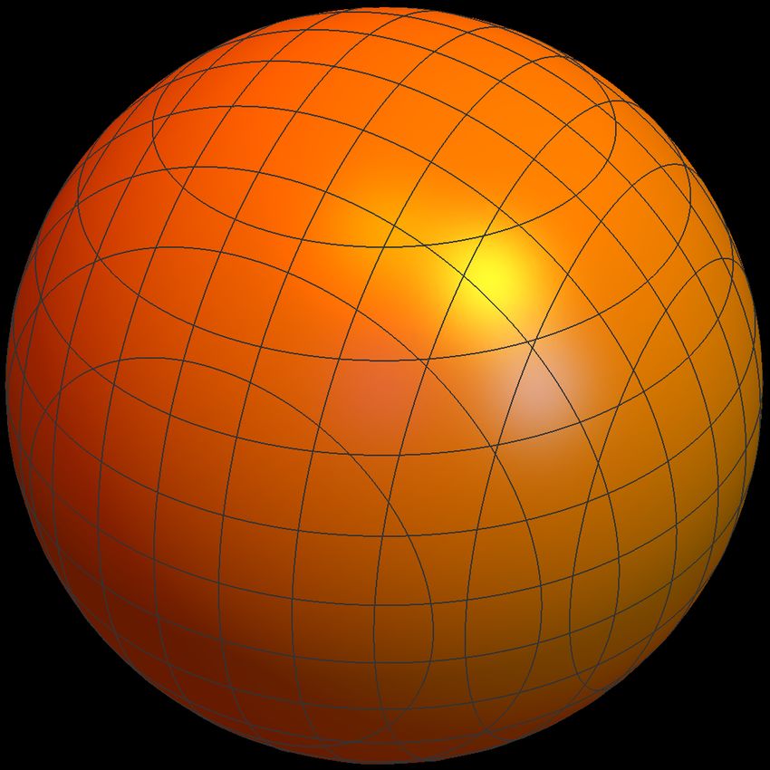
Österreichische Mathematische Gesellschaft

Gegründet 1903                          W. Imrich (MU Leoben)
http://www.oemg.ac.at/                  M. Kim (MathWorks)
email: oemg@oemg.ac.at                  M. Koth (Univ. Wien)
                                        M. Kraker (Graz)
Sekretariat:                            C. Krattenthaler (Univ. Wien)
                                        W. Müller (Univ. Klagenfurt)
Alpen-Adria-Universität Klagenfurt,
                                        H. Niederreiter (ÖAW)
Institut für Mathematik
                                        W. G. Nowak (Univ. Bodenkultur)
Universitätsstraße 65-67
                                        M. Oberguggenberger (Univ. Inns-
A-9020 Klagenfurt
                                        bruck)
email: oemg@oemg.ac.at
                                        W. Schachermayer (Univ. Wien)
                                        K. Sigmund (Univ. Wien)
Vorstand des Vereinsjahres 2021:
                                        H. Sorger (Wien)
B. Kaltenbacher (Univ. Klagenfurt):     R. Tichy (TU Graz)
Vorsitzende                             K. Unterkofler (FH Dornbirn)
J. Wallner (TU Graz):                   H. Zeiler (Wien)
Stellvertretender Vorsitzender
C. Fuchs (Univ. Salzburg):              Vorsitzende von Sektionen und
Herausgeber der IMN                     Kommissionen:
M. Ludwig (TU Wien):
                                        W. Woess (Graz)
Schriftführerin
                                        H.-P. Schröcker (Innsbruck)
M. Haltmeier (Univ. Innsbruck):
                                        C. Heuberger (Klagenfurt)
Stellvertretender Schriftführer
                                        F. Pillichshammer (Linz)
B. Lamel (Univ. Wien):
                                        S. Blatt (Salzburg)
Kassier
                                        I. Fischer (Wien)
P. Grohs (Univ. Wien):
                                        H. Humenberger (Didaktik-
Stellvertretender Kassier
                                        kommission)
E. Resmerita (Univ. Klagenfurt):
                                        W. Müller (Verantwortlicher für Ent-
Beauftragte für Frauenförderung
                                        wicklungszusammenarbeit)
C. Heuberger (Univ. Klagenfurt):
Beauftragter f. Öffentlichkeitsarbeit   Die Landesvorsitzenden und der Vor-
                                        sitzende der Didaktikkommission ge-
Beirat:                                 hören statutengemäß dem Beirat an.

A. Binder (Linz)                        Mitgliedsbeitrag:
M. Drmota (TU Wien)
H. Edelsbrunner (ISTA)                  Jahresbeitrag: 35,–
H. Engl (Univ. Wien)                    Bankverbindung: IBAN AT83-1200-
H. Heugl (Wien)                         0229-1038-9200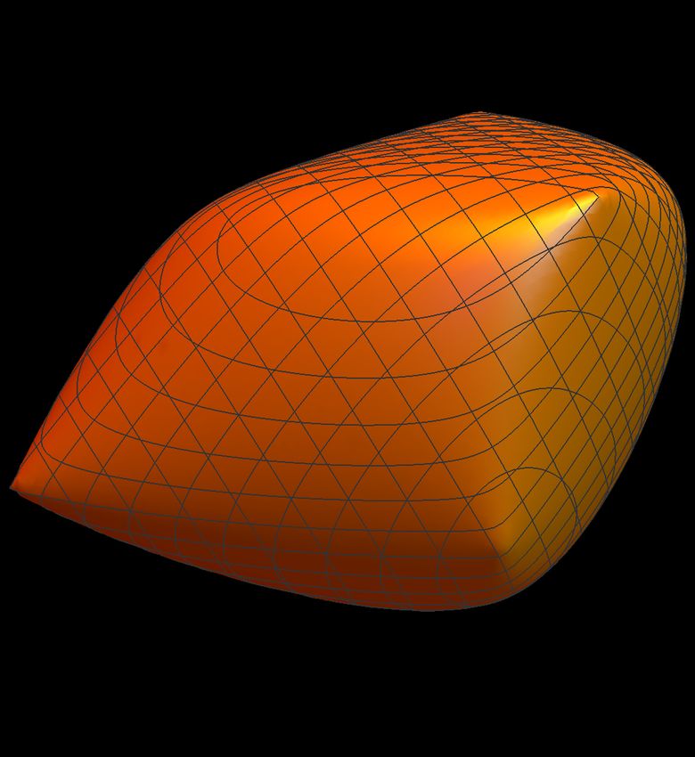
Internationale
                Mathematische
                Nachrichten
                International Mathematical News
                Nouvelles Mathématiques
                Internationales

                Nr. 246 (75. Jahrgang)                                April 2021

Inhalt
Gemma De las Cuevas and Tim Netzer: Quantum information theory and
free semialgebraic geometry: one wonderland through two looking glasses            1
Michael Missethan: Sparse random planar graphs         . . . . . . . . . . . . .   29
Michaela Szölgyenyi: Stochastic differential equations with irregular coef-
ficients: mind the gap! . . . . . . . . . . . . . . . . . . . . . . . . . . . .    43
Buchbesprechungen . . . . . . . . . . . . . . . . . . . . . . . . . . . . . .      57
Neue Mitglieder . . . . . . . . . . . . . . . . . . . . . . . . . . . . . . . .    59
Die Titelseite zeigt die epidemiologische Kurve von Covid-19 in Österreich im ersten Jahr der Pandemie. Die Daten stammen vom Dashboard der AGES. In die- sem Jahr wurde “flatten the curve” zu einem viel zitierten Schlagwort, die ef- fektive Reproduktionszahl, die 7-Tage-Inzidenz und andere Kennwerte sind einer informierten Öffentlichkeit nun bestens vertraut, exponentielles Wachstum ist für alle greifbarer geworden. In der Krise haben Mathematikerinnen und Mathema- tiker wichtige Sichtweisen beigesteuert und gemeinsam mit anderen Expertinnen und Experten somit einen wesentlichen Input für die Entscheidungen der Politik geliefert. Die Krise hat – so wie in allen Bereichen des Lebens – auch in der ma- thematischen scientific community für etliche Änderungen gesorgt. Videokonfe- renzen haben unseren Austausch geprägt. Offenbar geht es doch auch ohne Tafel, wenngleich die Diskussion und die Vermittlung von Ideen dabei gelitten hat! Es besteht die berechtigte Hoffnung, dass die gesundheitliche Gefahr mit der Imp- fung deutlich reduziert wird, sodass die sehr herausfordernden und schwierigen Pandemie-Monate dann letztlich hinter uns liegen werden.
Internat. Math. Nachrichten
                                                                         Nr. 246 (2021), 1–28

Quantum information theory and
free semialgebraic geometry: one
wonderland through two looking
glasses
Gemma De las Cuevas and Tim Netzer
University of Innsbruck

We illustrate how quantum information theory and free (i.e. noncommutative)
semialgebraic geometry often study similar objects from different perspectives.
We give examples in the context of positivity and separability, quantum magic
squares, quantum correlations in non-local games, and positivity in tensor net-
works, and we show the benefits of combining the two perspectives. This paper is
an invitation to consider the intersection of the two fields, and should be accessi-
ble for researchers from either field.

                                                                                     Live free or die.
                                                                            Motto of New Hampshire

1       Introduction
The ties between physics, computer science and mathematics are historically
strong and multidimensional. It has often happened that mathematical inven-
tions which were mere products of imagination (and thus thought to be useless
for applications) have later played a crucial role in physics or computer science.
A superb example is that of imaginary numbers and their use in complex Hilbert
spaces in quantum mechanics.1 Other examples include number theory and its
    1 Who   would have thought that the square root of −1 would have any physical relevance? See
[48].

ISSN 0020-7926 c 2021 Österr. Math. Gesellschaft
use in cryptography, or Riemannian geometry and its role in General Relativity. It is also true that physicists tend to be only aware of the mathematical tools useful for them — so there are many branches of mathematics which have not found an outlet in physics. The relevance of a statement depends on the glass through which we look at it. There are statements which are mathematically unimpressive but physically very impressive. A good example is entanglement. Mathematically, the statement that the positivity cone of the tensor product space is larger than the tensor product of the local cones is interesting, but not particularly wild or surprising. Yet, the physical existence of entangled particles is, from our perspective, truly remark- able. In other words, while the mathematics is easy to understand, the physics is mind-blowing. This is particularly true regarding Bell’s Theorem: while it is mathematically not specially deep, we regard the experimental violation of Bell inequalities [29, 33, 50] as very deep indeed. Another example is the no-cloning theorem — it is mathematically trivial, yet it has very far-reaching physical conse- quences. On the other hand, there are many mathematically impressive statements which are — so far — physically irrelevant. Finally, there are statements which can be both mathematically deep and central for quantum information theory, such as Stinespring’s Dilation Theorem. The goal of this paper is to illustrate how two relatively new disciplines in physics and mathematics — quantum information theory and free semialgebraic geometry — have a lot in common. ‘Free’ means noncommutative, because it is free of the commutation relation. So free semialgebraic geometry studies noncommutative versions of semialgebraic sets. On the other hand, quantum information theory is (mathematically) a noncommutative generalisation of classical information the- ory. So, intuitively, ‘free’ is naturally linked to ‘quantum’. Moreover, in both fields, positivity plays a very important role. Semialgebraic geometry examines questions arising from nonnegativity, like polynomial inequalities. In quantum information theory, quantum states are represented by positive semidefinite matri- ces. Positivity also gives rise to convexity, which is central in both fields, as we will see. So the two disciplines often study the same mathematical objects from different perspectives. As a consequence, they often ask different questions. For example, in quantum information theory, given an element of a tensor product space, one wants to know whether it is positive semidefinite, and how this can be efficiently represented and manipulated. In free semialgebraic geometry, the attention is focused on the geometry of the set of all such elements (see Table 1). We believe that much is to be learnt by bridging the gap among the two com- munities — in knowledge, notation and perspective. In this paper we hope to illustrate this point. This paper is thus meant to be accessible for physicists and mathematicians. 2
Quantum information theory             Free semialgebraic geometry
 Emphasis on the element                Emphasis on the set
 Given ρ = ∑α Aα ⊗ Bα , is it positive  Given {Aα }, characterise the set of
 semidefinite (psd)?                    {Bα } such that ∑α Aα ⊗ Bα is psd.
 Block positive matrices / Separable    Largest / smallest operator system
 psd matrices.                          over the psd cone.
 Every POVM can be dilated to a PVM.    The free convex hull of the set of
                                        PVMs is the set of POVMs.
 Can a correlation matrix p be realised Is p in the free convex hull of the free
 by a quantum strategy?                 independence model?
Table 1: Examples of the different approaches of quantum information theory and free
semialgebraic geometry in studying essentially the same mathematical objects. The vari-
ous notions will be explained throughout the paper.

Obviously we are not the first or the only ones to notice these similarities. In this
paper, however, we will mainly concentrate on what we have learnt from collab-
orating in recent years, and we will review a few other works. The selection of
other works is not comprehensive and reflects our partial knowledge. We also
remark that quantum information theory and free semialgebraic geometry are not
the only ones studying positivity in tensor product spaces. Compositional dis-
tributional semantics, for example, represents the meaning of words by positive
semidefinite matrices, and the composition of meanings is thus given by positivity
preserving maps — see e.g. [18, 11].
This article is organised as follows. We will first explain basic concepts in quan-
tum information theory and free semialgebraic geometry (Section 2) — the reader
familiar with them can skip the corresponding section. Then we will explain how
they are related (Section 3), and we will end with some closing words (Section 4).

2     Some basic concepts
Here we present some basic concepts in quantum information theory (Section 2.1)
and free semialgebraic geometry (Section 2.2).
Throughout the paper we denote the set of r × s complex matrices by Matr,s , the
set of r × r complex matrices by Matr , and we use the identification of Matr ⊗
Mats with Matrs . We will also often use the real subspace of Matr containing the
Hermitian elements, called Herr , and use that Herr ⊗ Hers is identified with Herrs .
The d-fold cartesian product of Herr is denoted Herdr .

                                                                                      3
2.1 Basic concepts from quantum information theory
Here we briefly introduce some concepts from quantum information theory. We
focus on finite-dimensional quantum systems of which we do not assume to have
perfect knowledge (in the language of quantum information, these are called
mixed states). See, e.g. [53, 43], for a more general overview.
The state of a quantum system is modelled by a normalized positive semidefinite
matrix, i.e. a
ρ ∈ Matd with ρ < 0 and tr(ρ) = 1,
where < 0 denotes positive semidefinite (psd), i.e. Hermitian with nonnegative
eigenvalues, and the trace, tr, is the sum of the diagonal elements. We reserve the
symbol > 0 for nonnegative numbers. A measurement on the system is modelled
by a positive operator valued measure (POVM), i.e. a set of psd matrices τi that
sum to the identity:
τ1 , . . . , τn ∈ Matd with all τi < 0 and ∑ τi = Id .
i
The probability to obtain outcome i on state ρ is given by
tr(ρτi ). (1)
Note that these probabilities sum to 1 because of the normalisation condition on
the τi ’s and ρ.
When the system is composed of several subsystems, the global state space is
modelled as a tensor product of the local spaces,
Matd = Matd1 ⊗ · · · ⊗ Matdn , (2)
where d = d1 · · · dn .
A state ρ is called separable (w.r.t. a given tensor product structure) if it can be
written as
r
(1) (n) ( j)
ρ = ∑ ρi ⊗ · · · ⊗ ρi with all ρi < 0.
i=1
This is obviously a stronger requirement than ρ being psd — not every ρ is sep-
arable. Separable states are not too interesting from a quantum information per-
spective: not separable states are called entangled, and entanglement is necessary
for many quantum information tasks.
4A quantum channel is the most general transformation on quantum states. Math-
ematically, it is modelled by a linear trace-preserving map
T : Matd → Mats
that is completely positive. Complete positivity means that the maps
idn ⊗ T : Matnd → Matns
are positive (i.e. map psd matrices to psd matrices) for all n, where idn is the
identity map on Matn .
Any linear map T : Matd → Mats is uniquely determined by its Choi matrix
d
CT := ∑ Ei j ⊗ T Ei j ∈ Matds ,
i, j=1
where Ei j is the matrix with a 1 in the (i, j)-position and 0 elsewhere.2 It is a
basic fact that T is completely positive if and only if CT is psd (see for example
[46, 54]). Moreover, a completely positive map T is entanglement-breaking [34]
if and only if CT is a separable matrix, and T is a positive map if and only if CT is
block positive, i.e.
tr((σ ⊗ τ)CT ) > 0 for all σ < 0, τ < 0.
Note that this is weaker than CT being psd, in which case tr(χCT ) > 0 for all χ < 0
(see Table 2). We also remark that this link between positivity notions of linear
maps and their Choi matrices does not involve the normalisation conditions on the
maps (e.g. preserving the trace) or the matrices (e.g. having a given trace).
Linear map Element in tensor product space
T : Matd → Mats ρ ∈ Matd ⊗ Mats
Entanglement-breaking map Separable matrix
Completely positive map Positive semidefinite matrix
Positive map Block positive matrix
Table 2: Correspondence between notions of positivity for linear maps and their Choi
matrices. Entanglement-breaking maps are a subset of completely positive maps, which
are a subset of positive maps. The same is true for the right column, of course.
2 If this is expressed in the so-called computational basis (which is one specific orthonormal
basis), this is written Ei j = |iih j| in quantum information.
52.2 Basic concepts from (free) semialgebraic geometry
We now introduce some basic concepts from free (i.e. noncommutative) semialge-
braic geometry. For a slightly more detailed introduction, see [41] and references
therein.
Our setup starts by considering a C-vector space V with an involution ∗. The two
relevant examples are, first, the case where V is the space of matrices and * is the
transposition with complex conjugation — denoted † in quantum information —,
and, second, Cd with entrywise complex conjugation.
The fixed points of the involution are called self-adjoint, or Hermitian, elements.
We denote the set of Hermitian elements of V by Vher . This is an R-subspace of
V , in which the real things happen.3
In the free setup, we do not only consider V but also higher levels thereof. Namely,
for any s ∈ N, we consider the space of s × s-matrices with entries over V ,
Mats (V ) = V ⊗ Mats .
Recall that Mats refers to s × s-matrices with entries over C. Mats (V ) is a C-
vector space with a ‘natural’ involution, consisting of transposing and applying ∗
entrywise. This thus promotes V and ∗ to an entire hierarchy of levels, namely
Mats (V ) for all s ∈ N with the just described involution.
We are now ready to define the most general notion of a free real set. This is
nothing but a collection
C = (Cs )s∈N
where each Cs ⊆ Mats (V )her =: Hers (V ). We call Cs the set at level s.
To make things more interesting, one often imposes conditions that connect the
levels. One important example is free convexity, which is defined as follows. For
any
τi ∈ Cti with i = 1, . . . , n,
and
n
vi ∈ Matti ,s with ∑ v∗i vi = Is, (3)
i=1
it holds that
n
∑ v∗i τivi ∈ Cs. (4)
i=1
Note that in (4) matrices over the complex numbers (namely vi ) are multiplied
with matrices over V (namely τi ). This is defined as matrix multiplication in the
3 Because it is where positivity and other interesting phenomena happen.
6usual way for v∗i τi vi , and using that elements of V can be multiplied with complex
numbers and added. For example, for n = 1, t = 2, s = 1, τ = (µi, j ) with µi, j ∈ V
for i = 1, 2, and v = (λ1 , λ2 )t with λi ∈ C, we have
v∗ τv = ∑ λ
¯ i λ j µi, j .
i, j
Note that if free convexity holds, then every Cs is a convex set in the real vector
space Hers (V ). But free convexity is generally a stronger condition than ‘classical’
convexity, as we will see.
In addition, a conic version of free convexity is obtained when giving up the nor-
malization condition on the vi , i.e. the right hand side of Eq. (3). In this case, C
is called an abstract operator system (usually with the additional assumption that
every Cs is a proper convex cone).
Now, free semialgebraic sets are free sets arising from polynomial inequalities.
This will be particularly important for the connection we hope to illustrate in
this paper. In order to define these, take V = Cd with the involution provided
by entrywise conjugation, so that Vher = Rd . Let z1 , . . . , zd denote free variables,
that is, noncommuting variables. We can imagine each zi to represent a matrix of
arbitrary size — later we will substitute zi by a matrix of a given size, and this
size will correspond to the level of the free semialgebraic set.
Now let ω be a finite word in the letters z1 , . . . , zd , that is, an ordered tuple of these
letters. For example, ω could be z1 z1 z4 or z4 z5 z4 . In addition, let σω ∈ Matm be
a matrix (of some fixed size m) that specifies the coefficients of word ω; this is
called the coefficient matrix. A matrix polynomial in the free variables z1 , . . . , zd
is an expression
p = ∑ σω ⊗ ω,
ω
where the sum is over all finite words ω, and where only finitely many coefficient
matrices σω are nonzero.
We denote the reverse of word ω by ω∗ . For example, if ω = z1 z2 z3 then ω∗ =
z3 z2 z1 . In addition, (σω )∗ is obtained by transposition and complex conjugation
of σω . If the coefficient matrices fulfill
(σω )∗ = σω∗ , (5)
then for any tuple of Hermitian matrices (τ1 , . . . , τd ) ∈ Herds we have that
p(τ1 , . . . , τd ) = ∑ σω ⊗ ω(τ1 , . . . , τd ) ∈ Herms .
ω
7That is, p evaluated at the Hermitian matrices τ1 , . . . , τd is a Hermitian matrix
itself.
So, for a given matrix polynomial p satisfying condition (5), we define the free
semialgebraic set at level s as the set of Hermitian matrices of size s such that p
evaluated at them is psd:
n o
d
Cs (p) := (τ1 , . . . , τd ) ∈ Hers | p(τ1 , . . . , τd ) < 0 .
Finally we define the free semialgebraic set as the collection of all such levels:
C (p) := (Cs (p))s∈N .
For example, let Eii denote the matrix with a 1 in entry (i, i) and 0 elsewhere. Then
the matrix polynomial
d
p = ∑ Eii ⊗ zi
i=1
defines the following free semialgebraic set at level s
n o
d
Cs (p) = (τ1 , . . . , τd ) ∈ Hers | E11 ⊗ τ1 + . . . + Edd ⊗ τd < 0 .
The positivity condition is equivalent to τi < 0 for all i, which gives this free set
the name free positive orthant. Note that for s = 1, the ‘free’ variables become
real numbers, n o
C1 (p) = (a1 , . . . , ad ) ∈ Rd | ai > 0 ∀i ,
which defines the positive orthant in d dimensions.
It is easy to see that any free semialgebraic set is closed under direct sums, mean-
ing that if (τ1 , . . . , τd ) ∈ Cs (p), (χ1 , . . . , χd ) ∈ Cr (p) then
(τ1 ⊕ χ1 , . . . , τd ⊕ χd ) ∈ Cr+s (p),
where τi ⊕ χi denotes the block diagonal sum of two Hermitian matrices. This is
because p(τ1 ⊕ χ1 , . . . τd ⊕ χd ) = p(τ1 , . . . τd ) ⊕ p(χ1 , . . . χd ), which is psd if and
only if each of the terms is psd.
Note also that a semialgebraic set is a Boolean combination of C1 (pi ) for a fi-
nite set of polynomials pi . A ‘free semialgebraic set’ is thus a noncommutative
generalisation thereof, with the difference that usually a single polynomial p is
considered.
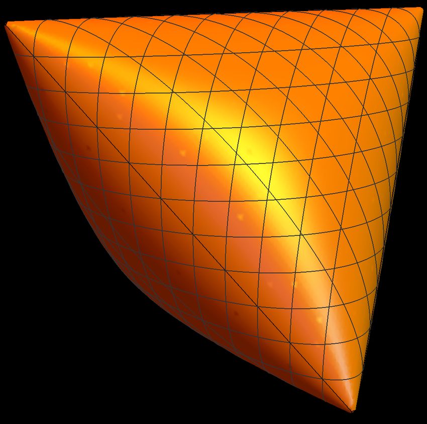
8Figure 1: Some three-dimensional spectrahedra taken from [42]. Spectrahedra are con-
vex sets described by a linear matrix inequality, and polyhedra are particular cases of
spectrahedra.
A very special case of free semialgebraic sets are free spectrahedra, which arise
from linear matrix polynomials. A linear matrix polynomial is a matrix polyno-
mial where every word ω depends only on one variable, i.e.
d
` = σ0 ⊗ 1 + ∑ σi ⊗ zi
i=1
with 1 being the empty word, and all σi ∈ Herm . The corresponding free set at
level s is given by
( )
d
Cs (`) = (τ1 , . . . , τd ) ∈ Herds | σ0 ⊗ Is + ∑ σi ⊗ τi < 0
i=1
and C (`) is called a free spectrahedron. The first level set,
n o
C1 (`) = (a1 , . . . , ad ) ∈ Rd | σ0 + a1 σ1 + · · · + ad σd < 0 ,
is known as a classical spectrahedron, or simply, a spectrahedron (see Fig. 1 for
some three-dimensional spectrahedra). If all σi are diagonal in the same basis,
then the spectrahedron C1 (`) becomes a polyhedron. (Intuitively, polyhedra have
flat facets whereas the borders of spectrahedra can be round, as in Fig. 1.) Thus,
every polyhedron is a spectrahedron, but not vice versa.
While the linear image (i.e. the shadow) of a polyhedron is a polyhedron, the
shadow of a spectrahedron needs not to be a spectrahedron. The forthcoming book
[42] presents a comprehensive treatment of spectrahedra and their shadows.4
3 One wonderland through two looking glasses
Let us now explain some recent results that illustrate how concepts and meth-
ods from the two disciplines interact. We will focus on positivity and separabil-
4 Shadows can be very different from the actual thing, as this shadow art by Kumi Yamashita
shows.
9ity (Section 3.1), quantum magic squares (Section 3.2), non-local games (Sec-
tion 3.3), and positivity in tensor networks (Section 3.4).
3.1 Positivity and separability
For fixed d, s ∈ N consider the set of states and separable states in Matd ⊗ Mats ,
namely Stated,s and Sepd,s , respectively. Both sets are closed in the real vector
space Herd ⊗ Hers . Moreover, both are semialgebraic, since Stated,s is a classical
spectrahedron, and Sepd,s can be proven to be semialgebraic using the projection
theorem/quantifier elimination in the theory of real closed fields (see, e.g., [47]).
It has long been known that Sepd,s is a strict subset of Stated,s whenever d, s > 1. A
recent work by Fawzi [26], building on Scheiderer’s [49], strengthens this result,
by showing that the geometry of these two sets is significantly different:
Theorem 1 ([26]). If d + s > 5 then Sepd,s is not a spectrahedral shadow.
Recall that a spectahedral shadow is the linear image of a spectrahedron.
Together with the relations of Table 2, it follows from the previous result that the
corresponding sets of linear maps T : Matd → Mats satisfy that:
(i) Entanglement-breaking maps form a convex semialgebraic set which is not
a spectrahedral shadow,
(ii) Completely positive maps form a spectrahedron, and
(iii) Positive maps form a convex semialgebraic set which is not a spectra-
hedral shadow. This follows from (i), the duality of positive maps and
entanglement-breaking maps, and the fact that duals of spectrahedral shad-
ows are also spectrahedral shadows [42].
Let us now consider the set of states and separable states as free sets. Namely, for
fixed d > 1 let
Stated := Stated,s s∈N and Sepd := Sepd,s s∈N .
This is a particular case of the setup described above, where V = Matd and the
involution is provided by †. Moreover, both sets satisfy the condition of free
convexity (Eq. (4)). In addition, Stated is a free spectrahedron, whereas Sepd is
not, since for fixed s it is not even a classical spectrahedral shadow at level s due
to Theorem 1.
Viewing states as free sets also leads to an easy conceptual proof of the following
result [13], which was first proven by Cariello [8].
10Theorem 2 ([13, 8]). For arbitrary d, s ∈ N, if ρ ∈ Stated,s is of tensor rank 2, i.e.
it can be written as
ρ = σ1 ⊗ τ1 + σ2 ⊗ τ2 , (6)
where σi and τi are Hermitian, then it is separable.
Note that σi and τi need not be psd. Let us sketch the proof of [13] to illustrate the
method.
Proof. Consider the linear matrix polynomial ` = σ1 ⊗ z1 + σ2 ⊗ z2 , where σ1 , σ2
are given in Eq. (6). The fact that ρ is a state means that the corresponding free
set of level s contains (τ1 , τ2 ):
(τ1 , τ2 ) ∈ Cs (`).
At level one, the spectrahedron C1 (`) is a convex cone in R2 . A convex cone in the
plane must be a simplex cone, i.e. a cone whose number of extreme rays equals the
dimension of the space. In R2 this means that the cone is spanned by two vectors,
C1 (`) = cone{v1 , v2 },
where v1 , v2 ∈ R2 . When the cone at level one is a simplex cone, the free convex
cone is fully determined [25, 27].
In addition, the sets
Ts := {v1 ⊗ η1 + v2 ⊗ η2 | 0 4 ηi ∈ Hers }
also give rise to a free convex cone (Ts )s∈N , and we have that T1 = C1 (`).
These two facts imply that Ts = Cs (`) for all s ∈ N. Using a representation for
(τ1 , τ2 ) in Ts , and substituting into Eq. (6) results in a separable decomposition of
ρ.
The crucial point in the proof is that when the cone at level one is a simplex cone,
the free convex cone is fully determined. This is not a very deep insight — it can
easily be reduced to the case of the positive orthant, where it is obvious.
Note that the separable decomposition of ρ obtained in the above proof contains
only two terms — in the language of [13, 21], ρ has separable rank 2.
11References [6, 7] also propose to use free spectrahedra to study some problems in
quantum information theory, but from a different perspective. Given d Hermitian
matrices σ1 , . . . , σd ∈ Herm , one would like to know whether they fulfill
0 4 σi 4 Im ,
because this implies that each σi gives rise to the binary POVM consisting of
σi , Im − σi . In addition, one would like to know whether σ1 , . . . , σd are jointly
measurable, meaning that these POVMs are the marginals of one POVM (see [6]
for an exact definition).
Now use σ1 , . . . , σd to construct the linear matrix polynomial
d
` := Im ⊗ 1 − ∑ (2σi − Im ) ⊗ zi
i=1
and consider its free spectrahedron C (`) = (Cs (`))s∈N . Define the matrix diamond
as the free spectrahedron D = (Ds )s∈N with
( )
d
Ds := (τ1 , . . . , τd ) ∈ Herds | Is − ∑ ±τi < 0 ,
i=1
where all possible choices of signs ± are taken into account. Note that D1 is just
the unit ball of Rd in 1-norm, which explains the name diamond. Note also that
D1 ⊆ S1 (`) is equivalent to 0 4 σi 4 Im for all i = 1, . . . , d. Since these finitely
many conditions can be combined into a single linear matrix inequality (using
diagonal blocks of matrix polynomials), D is indeed a free spectrahedron. The
following result translates the joint measurability to the containment of free spec-
trahedra:
Theorem 3 ([6]). σ1 , . . . , σd are jointly measurable if and only if D ⊆ C (`).
That one free spectrahedron is contained in another, D ⊆ C (`), means that each
of their corresponding levels satisfy the same containment, i.e. Ds ⊆ Cs (`) for all
s ∈ N.
The containment of spectrahedra and free spectrahedra has received considerable
attention recently [4, 31, 32, 27, 45]. One often studies inclusion constants for
containment, which determine how much the small spectrahedron needs to be
shrunk in order to obtain inclusion. In [6, 7] this is used to quantify the degree of
incompatibility, and to obtain lower bounds on the joint measurability of quantum
measurements.
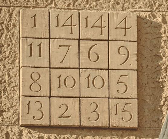
12Figure 2: (Left) The magic square on the façade of the Sagrada Família in Barcelona,
where every row and column adds to 33. (Right) The magic square in Albrecht Dürer’s
lithograph Melencolia I, where every row and column adds to 34.
3.2 Quantum magic squares
Let us now look at magic squares and their quantum cousins.
A magic square is a d × d-matrix with positive entries such that every row and
column sums to the same number (see Fig. 2 for two beautiful examples.) A
doubly stochastic matrix is a d × d-matrix with real nonnegative entries, in which
each row and each column sums to 1. So doubly stochastic matrices contain a
probability measure in each row and each column. For example, dividing every
entry of Dürer’s magic square by 34 results in a doubly stochastic matrix. Now,
the set of doubly stochastic matrices forms a polytope, whose vertices consist of
the permutation matrices, i.e. doubly stochastic matrices with a single 1 in every
row and column and 0 elsewhere (that is, permutations of the identity matrix).
This is the content of the famous Birkhoff–von Neumann Theorem.
A ‘quantum’ generalization of a doubly stochastic matrix is obtained by putting a
POVM (defined in Section 2.1) in each row and each column of a d × d-matrix.
This defines a quantum magic square [14]. That is, in passing from doubly
stochastic matrices to quantum magic squares, we promote the nonnegative num-
bers to psd matrices. The normalisation conditions on the numbers (that they
sum to 1) become the normalisations of the POVM (that they sum to the identity
matrix).
What is a quantum generalisation of a permutation matrix? Permutation matrices
only contain 0s and 1s, so in passing to the quantum version, we promote 0 and
1 to orthogonal projectors (given that 0 and 1 are the only numbers that square
to themselves). The relevant notion is thus that of a projection valued measure
(PVM), in which each measurement operator τ1 , . . . , τd is an orthogonal projec-
tion, τ2i = τi . Quantum permutation matrices are magic squares containing a PVM
13in each row and column [2].5
While PVMs are a special case of POVMs, every POVM dilates to a PVM (see,
e.g., [46]):
Theorem 4 (Naimark’s Dilation Theorem). Let τ1 , . . . , τd (of size m × m) form a
POVM. Then there exists a PVM σ1 , . . . , σd (of size n × n, for some n) and a matrix
v ∈ Matn,m such that
v∗ σi v = τi for all i = 1, . . . , d.
In terms of free sets, this theorem states that the free convex hull of the set of PVMs
is precisely the set of POVMs. Both sets are free semialgebraic, and the POVMs
even form a free spectrahedron.
Through the glass of free semialgebraic geometry, quantum magic squares form
a free spectrahedron over the space V = Matd , equipped with entrywise complex
conjugation as an involution. Level s corresponds to POVMs with matrices of size
s × s, and thus level 1 corresponds to doubly stochastic matrices. We thus recover
the magic in the classical world at level 1, and we have an infinite tower of levels
on top of that expressing the quantum case.
Furthermore, quantum permutation matrices form a free semialgebraic set whose
first level consists of permutation matrices. The ‘classical magic’ is thus again
found at level 1, and the quantum magic is expressed in an infinite tower on top
of it.
Now, recall that the Birkoff–von Neumann Theorem says that the convex hull of
the set of permutation matrices is the set of doubly stochastic matrices. So the per-
mutation matrices are the vertices of the polytope of doubly stochastic matrices.
In the light of the towers of quantum magic squares and quantum permutation ma-
trices, this theorem fully characterises what happens at level one. We ask whether
a similar characterisation is possible for the quantum levels: Is the free convex hull
of quantum permutation matrices equal to the set of quantum magic squares?
This question can be phrased in terms of dilations as follows. By Naimark’s Di-
lation Theorem we know that every POVM dilates to a PVM. The question is
whether this also holds for a two-dimensional array of POVMs, i.e. whether every
square of POVMs can dilated to a square of PVMs. The non-trivial part is that the
dilation must work simultaneously for all POVMs in the rows and columns. The
two-dimensional version of Naimark’s Dilation Theorem can thus be phrased as:
Does every quantum magic square dilate to a quantum permutation matrix?
The answer to these questions is ‘no’: these quantum generalisations fail to be
true in the simplest nontrivial case. This means that there must exist very strange
(and thus very interesting) quantum magic squares:
5 See
the closely related notion of quantum Latin squares [37, 35], which in essence are quan-
tum permutation matrices with rank 1 projectors.
14Theorem 5 ([14]). For each d > 3, the free convex hull of the free semialgebraic
set of d × d quantum permutation matrices is strictly contained in the free spec-
trahedron of quantum magic squares. This strict containment already appears at
level s = 2.
The latter statement means that there is a d × d-matrix with POVMs of size 2 × 2
in each row and column which does not dilate to a matrix with a PVM in each row
and column.
In other words, the tower of quantum levels does not admit the same kind of
‘easy’ characterisation as level one or the case of a single POVM — at least not
the natural generalisations we have considered here. This is yet another sign of
the richer structure of the quantum world compared to the classical one.
3.3 Non-local games and quantum correlations
Consider a game with two players, Alice and Bob, and a referee. The referee
chooses a question randomly from finite sets QA and QB for Alice and Bob, re-
spectively, and sends them to Alice and Bob. Upon receiving her question, Alice
chooses from a finite set AA of answers, and similarly Bob chooses his answer
from the finite set AB . They send their answers to the referee, who computes a
winning function
w : QA × QB × AA × AB → {0, 1}
to determine whether they win or lose the game (value of w being 1 or 0, respec-
tively).
During the game, Alice and Bob know both the winning function w and the prob-
ability measure on QA × QB used by the referee to choose the questions. So be-
fore the game starts Alice and Bob agree on a joint strategy. However, during
the game Alice and Bob are ‘in separate rooms’ (or in separate galaxies) so they
cannot communicate. In particular, Alice will not know Bob’s question and vice
versa. In order to find the strategy that maximises the winning probability, Alice
and Bob have to solve an optimisation problem.6
What kind of strategies may Alice and Bob choose? It depends on the resources
they have. First, in a classical deterministic strategy, both Alice and Bob reply
deterministically to each of their questions, and they do so independently of each
other. This is described by two functions
cA : QA → AA and cB : QB → AB ,
which specify which answer Alice and Bob give to each question.
6 Thus, strictly speaking, this is not a game in the game-theoretic sense, but (just) an optimisa-
tion problem.
15Slightly more generally, in a classical randomised strategy, Alice and Bob’s an-
swers are probabilistic, but still independent of each other. This is described by
rA : QA → Pr(AA ) and rB : QB → Pr(AB ),
where Pr(S) denotes the set of probability measures on the set S. Namely, if Alice
receives question a, the probability that she answers x is given by rA (a)(x), where
rA (a) is the probability measure on AA corresponding to question a. Similarly,
Bob answers y to b with probability rB (b)(y). Since Alice and Bob answer inde-
pendently of each other, the joint probability of answering x, y upon questions a, b
is the product of the two,
p(x, y | a, b) = rA (a)(x) · rB (b)(y). (7)
Finally, a quantum strategy allows them to share a bipartite state ρ ∈ Stated,s . The
questions determine which measurement to apply to their part of the state, and the
measurement outcomes determine the answers. This is described by functions
qA : QA → POVMd (AA ) and qB : QB → POVMs (AB ) (8)
whose image is the set of POVMs with matrices of size d × d and s × s, respec-
tively, on the respective sets of answers. The probability that Alice answers x
upon receiving a is described by qA (a)(x), which is the psd matrix that the POVM
qA (a) assigns to answer x. Similarly, Bob’s behaviour is modelled by qB (b)(y).
Since they act independently of each other, this is described by the tensor product
of the two. Using rule (1), we obtain that their joint probability is given by
p(x, y | a, b) = tr (ρ (qA (a)(x) ⊗ qB (b)(y))) . (9)
Now, the table of conditional probabilities
(p(x, y | a, b))(a,b,x,y)∈QA ×QB ×AA ×AB
is called the correlation matrix of the respective strategy. For any given kind of
strategy, the set of correlation matrices is the feasible set of the optimisation prob-
lem that Alice and Bob have to solve. The objective function of this optimisation
problem is given by the winning probability. Since this objective function is lin-
ear in the correlation matrix entries, one can replace the feasible set by its convex
hull.
The important fact is that quantum strategies cannot be reproduced by classical
randomised strategies:
Theorem 6 ([3, 10]). If at least 2 questions and 2 answers exist for both Alice and
Bob, the convex hull of correlation matrices of classical randomised strategies is
strictly contained in the set of correlation matrices of quantum strategies.
16For classical randomised strategies, passing to the convex hull has the physical
interpretation of including a hidden variable. The latter is a variable whose value
is unknown to us, who are describing the system, and it is usually denoted λ.
However, this mysterious variable λ is shared between Alice and Bob, and it will
determine the choice of their POVMs together with their respective questions a, b.
This is the physical interpretation of the convex hull
p(x, y | a, b) = ∑ qλ rA (a, λ)(x) · rB (b, λ)(y),
λ
where qλ is the probability of the hidden variable taking the value λ. For example,
we can imagine that Alice and Bob are listening to a radio station which plays
songs from a certain list, but this is a ‘private’ radio station to which we have no
access. The song at the moment of playing the game (i.e. receiving the questions)
will determine the value of λ (i.e. λ is an index of that list).
Theorem 6 thus states that quantum strategies cannot be emulated by classical
strategies, even if we take into account ‘mysterious’ hidden variables.
Let us now approach these results from the perspective of free sets. Assume for
simplicity that all four sets QA , QB , AA , AB have two elements. A quantum strategy
consists of a state ρ ∈ Stated,s and the following psd matrices for Alice and Bob,
respectively, satisfying this normalisation condition:
(i) (i)
σ j < 0 and τ j < 0
(i) (i) (10)
such that ∑σj = Id and ∑τj = Is ,
j j
where i, j = 1, 2. The superscript refers to the questions and the subscript to the
answers. The correlation matrix is given by
(i) ( j)
tr ρ σk ⊗ τl .
i, j,k,l
Using the spectral decomposition of ρ = ∑r vr v∗r , it can be written as
∗ (i) ( j)
∑ vr σk ⊗ τl vr , (11)
r i, j,k,l
where vr ∈ Cd ⊗ Cs and ∑r v∗r vr = 1. Through the looking glass of free semialge-
braic geometry, this is first level of a free convex hull. To see this, define the free
17set I as
[ (i) ( j) (i) ( j)
I= σk ⊗ τ l ∈ Mat4 (Matd ⊗ Mats ) | σk and τl satisfy (10)
i, j,k,l
d,s≥1
(12)
(Note that the 4 is due the fact that we have 2 questions and 2 answers; more
generally we would have a matrix of size |QA ||QB | × |AA ||AB |. Note also that the
ordering of questions and answers of Alice and Bob is irrelevant for the following
discussion.)
If we look at level 1 of this free set, we encounter that I1 is the subset of Mat4 (R)
consisting precisely of the correlation matrices of classical randomized strategies.
In other words, when d = s = 1, the formula coincides with that of (7). Further-
more, higher levels of this free set contain the tensor products of POVMs of Alice
and Bob in the corresponding space Matd and Mats . Since I1 is called the indepen-
dence model in algebraic statistics [23], we call I the free independence model,
since this is the natural noncommutative generalisation of independent strategies.
Let us now consider the free convex hull of I . First of all, computing the con-
ditional probabilities of a pair of POVMs with a given state ρ corresponds to
compressing to level 1 with the vectors {vr } given by the spectral decomposition
of ρ, as in (11). So the set of quantum correlations is the first level of the free
convex hull of the free independence model.
We thus encounter an interesting phenomenon: the free convex hull of a free set
can be larger than the classical convex hull at a fixed level. Specifically, the convex
hull of I1 is the set of classical correlations, whereas the free convex hull of I at
level 1 is the set of quantum correlations, which are different by Theorem 6. In
fact, wilder things can happen: fractal sets can arise in the free convex hull of free
semialgebraic sets [1]. We wonder what these results imply for the corresponding
quantum information setup.
Now, in the free convex hull of I , what do higher levels correspond to? Com-
pressing to lower levels (i.e. with smaller ds) corresponds to taking the partial
trace with a psd matrix of size smaller than ds. This results in 4 psd matrices (one
for each i, j, k, l), each of size < ds, which do not need to be an elementary tensor
product.
What about ‘compressing’ to higher levels? Any compression to a higher level can
be achieved by direct sums of the POVMs of Alice and Bob and a compression to
a lower level as we just described. The number of elements in this direct sum is
precisely n in (4). Another way of seeing that the direct sum is needed is by noting
that, if n = 1, the matrices vi cannot fulfill the normalisation condition on the right
hand side of (4). In quantum information terms, this says that a POVM in a given
dimension cannot be transformed to a POVM in a larger dimension by means of
an isometry, because the terms will sum to a projector instead of the identity.
18Let us make two final remarks. The first one is that I is not a free semialge-
braic set, for the simple reason that it is not closed under direct sums (which is a
property of these sets, as we saw in Section 2.2), as is easily checked.
The second remark is that the free convex hull of the free independence model is
not closed. This follows from the fact that, at level 1, this free convex hull fails to
be closed, as shown in [51] and for smaller sizes in [24].
Theorem 7 ([51, 24]). For at least 5 questions and 2 answers, the set of quantum
correlation matrices is not closed.
In our language, this implies that the level ds — which is to be compressed to
level 1 in the construction of the free convex hull — cannot be upper bounded.
That is, the higher ds, the more things we will obtain in its compression to level
1.
In the recent preprint [28] the membership problem in the closure of the set of
quantum correlations is shown to be undecidable, for a fixed (and large enough)
size of the sets of questions and answers.
A computational approach to quantum correlations, comparable to sums-of-
squares and moment relaxation approaches in polynomial optimisation [5, 42],
is the NPA hierarchy [38, 39, 40]. We briefly describe the approach here, omitting
technical details. Assume one is given a table
p = (p(x, y | a, b))(a,b,x,y)∈QA ×QB ×AA ×AB ,
and the task is to check whether it is the correlation matrix of a quantum strategy.
The NPA hierarchy provides a family of necessary conditions, each more stringent
than the previous one, for p to be a quantum strategy.
In order to understand the NPA hierarchy, we will first assume that p is a correla-
tion matrix, i.e. there is a state ρ and strategies such that (9) holds. We will use this
state and strategies to define a positive functional on a certain algebra. Namely,
we consider the game ∗-algebra
G := ChQA × AA , QB × AB i.
This is an algebra of polynomials in certain noncommuting variables. Explicitly,
for each question and answer pair from Alice and Bob, (a, x) and (b, y), there
is an associated self-adjoint variable, z(a,x) and z(b,y) , respectively. G consists
of all polynomials with complex coefficients in these variables; for example, the
19monomial z(a,x) z(b,y) ∈ G . Now, if we had the strategy ρ, qA , qB we could construct
a linear functional
ϕ: G → C
by evaluating the variables z(a,x) and z(b,y) at the psd matrices qA (a)(x) ⊗ Is and
Id ⊗ qB (b)(y), respectively, and computing the trace inner product with the state
ρ. So, in particular, evaluating ϕ at the monomial z(a,x) z(b,y) would yield
ϕ(z(a,x) z(b,y) ) = tr (ρ ((qA (a)(x) ⊗ Is ) · (Id ⊗ qB (b)(y)))) (13)
= p(x, y | a, b). (14)
The crucial point is that ϕ evaluated at this monomial needs to have the value
p(x, y | a, b) for any strategy realising p. In other words, the linear constraint
on ϕ expressed in Equation (14) must hold even if we do not know the strategy.
This functional must satisfy other nice properties independently of the strategy
too, such as being positive.
This perspective is precisely the one we now take. Namely, we assume that the
strategy ρ, qA , qB is not given (since our question is whether p is a quantum strat-
egy at all), and we search for a functional on G that has the stated properties (or
other properties, depending on the kind of strategies one is looking for). When re-
stricted to a finite-dimensional subspace of G , this becomes a semidefinite optimi-
sation problem, as can be easily checked. The dimension of this subspace will be
the parameter indicating the level of the hierarchy, which is gradually increased.
Solvability of all these semidefinite problems is thus a necessary condition for p
to be a quantum correlation matrix. In words, the levels of the NPA hierarchy
form an outer approximation to the set of correlations. Conversely, if all/many of
these problems are feasible, one can apply a (truncated) Gelfand-Naimark-Segal
(GNS) construction (see for example [46]) to the obtained functional, and thereby
try to construct a quantum strategy that realises p. This is the content of the NPA
hierarchy from the perspective of free semialgebraic geometry.
3.4 Positivity in tensor networks
Let us finally explain some results about positivity in tensor networks. The results
are not as much related to free semialgebraic geometry as to positivity and sums
of squares, as we will see.
Since the state space of a composite quantum system is given by the tensor product
of smaller state spaces (Eq. (2)), the global dimension d grows exponentially with
the number of subsystems n. Very soon it becomes infeasible to work with the
entire space — to describe n = 270 qubits di = 2, we would need to deal with a
space dimension d ∼ 2270 ∼ 1080 , the estimated number of atoms in the Universe.
To describe anything at the macro-scale involving a mole of particles, ∼ 1023 , we
2023
would need a space dimension of ∼ 210 , which is much larger than a googol
100
(10100 ), but smaller than a googolplex (1010 ). These absurd numbers illustrate
how quickly the Hilbert space description becomes impractical — in practice, it
works well for a few tens of qubits.7
Fortunately, many physically relevant states admit an efficient description. The
ultimate reason is that physical interactions are local (w.r.t. a particular tensor
product decomposition; this decomposition typically reflects spatial locality). The
resulting relevant states admit a description using only a few terms for every local
Hilbert space. The main idea of tensor networks is precisely to use a few matrices
for every local Hilbert space Matdi (Eq. (2); see, e.g., [44, 9]).
Now, this idea interacts with positivity in a very interesting way. Positivity is a
property in the global space Matd which cannot be easily translated to positiv-
ity properties in the local spaces. As we will see, there is a ‘tension’ between
using a few matrices for each local Hilbert space and representing the positivity
locally. This mathematical interplay has implications for the description of quan-
tum many-body systems, among others.
Let us see one example of a tensor network decomposition where this positivity
problem appears. To describe a mixed state in one spatial dimension with periodic
boundary conditions we use the matrix product density operator form (MPDO) of
ρ,
r
(1) (2) (n)
ρ= ∑ ρi1 ,i2 ⊗ ρi2 ,i3 ⊗ · · · ⊗ ρin ,i1 .
i1 ,...,in =1
The smallest such r is called the operator Schmidt rank of ρ [52, 55]. Clearly,
every state admits an MPDO form, and the ones with small r can be handled
efficiently. But how is the positivity of ρ reflected in the local matrices? Clearly, if
(k)
all local matrices are psd (i.e. ρi j < 0) then ρ will be psd. But some sums of non-
psd matrices will also give rise to a global psd matrix, since negative subspaces
may cancel in the sum. Can one easily characterise the set of local matrices whose
sum is psd? The short answer is ‘no’.
For further reference, if all local matrices are psd, so that ρ is separable, the cor-
responding r is called the separable rank of ρ [21, 17].
To obtain a local certificate of positivity, we first express ρ = ξξ∗ (which is pos-
sible only if ρ is psd) and then apply the tensor network ‘philosophy’ to ξ, i.e.
express ξ as an MPDO:
r
∗ (1) (2) (n)
ρ = ξξ with ξ= ∑ ξi1 ,i2 ⊗ ξi2 ,i3 ⊗ · · · ⊗ ξin ,i1 .
i1 ,...,in =1
7 The lack of scalability of this description is far from being a unique case in physics — most
theories are not scalable. One needs to find the new relevant degrees of freedom at the new scale,
which will define an emergent theory.
21This is the local purification form of ρ. Note that there are many ξ that satisfy
ρ = ξξ∗ , as ξ needs not to be Hermitian or a square matrix (it could be a column
vector). The smallest r among all such ξ is called the purification rank of ρ.
The interesting point for the purposes of this paper is that the purification rank is a
noncommutative generalisation of the positive semidefinite rank of a nonnegative
matrix. There are many more such connections: the separable rank, the transla-
tional invariant (t.i.) purification rank, and the t.i. separable rank are noncommu-
tative generalisations of the nonnegative rank, the cpsd rank and the cp rank of
nonnegative matrices, respectively [21]. As a matter of fact, this connection holds
in much greater generality, as we will explain below. In all of these cases, the
ranks coincide for quantum states that are diagonal in the computational basis.
From our perspective, this connection is beneficial for both sides. For example,
for quantum many-body systems, this insight together with the results by [30]
leads to the following result:
Theorem 8 ([22, 21]). The purification rank cannot be upper bounded by a func-
tion of the operator Schmidt rank only. The separable rank cannot be upper
bounded by a function of the purification rank only.
(It is worth noting these separations are not robust, as they disappear in the ap-
proximate case for certain norms [19].)
Conversely, the quantum perspective provides a natural and well-motivated path
for generalisation of the ‘commutative’ results about cpsd rank, cp rank, etc. For
example, in [30] it is shown that the extension complexity of a polytope w.r.t. a
given cone is given by the rank of the slack matrix of that polytope w.r.t. that cone.
We wonder whether this result could be a generalisation to the noncommutative
world. This would give a geometric interpretation of the purification rank, the
separable rank and their symmetric versions, perhaps as extension complexities
of some objects.
Symmetry is a central property in physics, both conceptually and practically. Con-
ceptually, symmetry is the other side of the coin of a conserved quantity (by
Noether’s Theorem). Practically, it allows for more efficient mathematical de-
scriptions, as symmetric objects have fewer degrees of freedom. For example,
in the above context, ρ is translational invariant if it remains unchanged under
cyclic permutations of the local systems. This raises the question: is there an
MPDO form that explicitly expresses this symmetry? For example, the following
form does,
r
ρ= ∑ ρi1 ,i2 ⊗ ρi2 ,i3 ⊗ · · · ⊗ ρin ,i1 ,
i1 ,...,in =1
22because it uses the same matrices on every site, and the arrangement of indices is
such that a cyclic permutation of the local systems does not change ρ. But does
this hold for other symmetries too?
The existence of such invariant decompositions and their corresponding ranks has
been studied in a very general framework [17]. Explicitly, every tensor decompo-
sition is represented as a simplicial complex, where the individual tensor product
spaces are associated to the vertices, and the summation indices to the facets. The
symmetry is modelled by a group action on the simplicial complex. The central
result is that an invariant decomposition exists if the group action is free on the
simplicial complex [17]. Just to give one example, if ρ ∈ Matd ⊗Matd is separable
and symmetric, it will in general not admit a decomposition of the type
ρ = ∑ ρα ⊗ ρα with all ρα psd,
α
but it will have one of the type
ρ = ∑ ρα,β ⊗ ρβ,α with all ρα,β psd.
α,β
From the perspective of our framework, this is due to the fact that the group per-
muting the two end points of an edge does not act freely on the edge connecting
them. But this group action can be made free if the two points are connected by
two edges, leading to the two indices α, β in the above sum. This is one example
of a refinement of a simplicial complex, which makes the action of the group free
[17].
Finally, we remark that this framework of tensor decompositions with invariance
can not only be applied to quantum-many body systems, but to any object in a
tensor product space. One example are multivariate symmetric polynomials with
positivity conditions [20].
A related question is the existence of invariantdecompositions uniform in the
system size. Namely, given a tensor ρ = ρα,β α,β=1,...,r with all ρα,β ∈ Matd ,
define
r
τn (ρ) := ∑ ρα1 ,α2 ⊗ ρα2 ,α3 ⊗ · · · ⊗ ραn ,α1 ∈ Matd n
i1 ,...,in =1
for all n ∈ N. The result, in this case, is very different from the fixed n case:
Theorem 9 ([12]). Let d, r > 7. Then it is undecidable whether τn (ρ) < 0 for all
n ∈ N.
23Sie können auch lesen