The effect of bathymetric modification on water age in the Elbe Estuary

Article, Published Version

Holzwarth, Ingrid; Weilbeer, Holger; Wirtz, Kai W.
The effect of bathymetric modification on water age in the
Elbe Estuary
Die Küste
Zur Verfügung gestellt in Kooperation mit/Provided in Cooperation with:
Kuratorium für Forschung im Küsteningenieurwesen (KFKI) (Hg.)

Verfügbar unter/Available at: https://hdl.handle.net/20.500.11970/107397

Vorgeschlagene Zitierweise/Suggested citation:
Holzwarth, Ingrid; Weilbeer, Holger; Wirtz, Kai W. (2019): The effect of bathymetric
modification on water age in the Elbe Estuary. In: Die Küste 87. Karlsruhe: Bundesanstalt für
Wasserbau. S. 261-282. https://doi.org/10.18171/1.087109.

Standardnutzungsbedingungen/Terms of Use:

Die Dokumente in HENRY stehen unter der Creative Commons Lizenz CC BY 4.0, sofern keine abweichenden
Nutzungsbedingungen getroffen wurden. Damit ist sowohl die kommerzielle Nutzung als auch das Teilen, die
Weiterbearbeitung und Speicherung erlaubt. Das Verwenden und das Bearbeiten stehen unter der Bedingung der
Namensnennung. Im Einzelfall kann eine restriktivere Lizenz gelten; dann gelten abweichend von den obigen
Nutzungsbedingungen die in der dort genannten Lizenz gewährten Nutzungsrechte.
Documents in HENRY are made available under the Creative Commons License CC BY 4.0, if no other license is
applicable. Under CC BY 4.0 commercial use and sharing, remixing, transforming, and building upon the material
of the work is permitted. In some cases a different, more restrictive license may apply; if applicable the terms of
the restrictive license will be binding.

Die Küste, 87, 2019 https://doi.org/10.18171/1.087109

The effect of bathymetric modification on water age
in the Elbe Estuary
Ingrid Holzwarth1, Holger Weilbeer1 and Kai W. Wirtz2
1 Bundesanstalt für Wasserbau
2 Helmholtz-Zentrum Geesthacht

Summary
The transport time of substances is a physical factor that influences the completeness of
biogeochemical reactions in the estuary. Since hydrodynamic changes induce changes in
transport time, river discharge and its seasonal variability strongly determine the transport
time of riverine water and its fluctuations.
A factor that leads to a permanent change in hydrodynamics is man-made bathymetric
modification. However, the impact of such modification on transport time has never been
quantified. Here we show for the Elbe Estuary (Germany), an example of a partially to
well-mixed alluvial estuary, that the impact of typical, decadal man-made bathymetric mod-
ification on the transport time of riverine water is much smaller than the effect of the
natural variability in river discharge. In this study, we used riverine water age to determine
transport time. We found the age difference due to river discharge variation to be in the
order of days to weeks, depending on the location within the estuary. In contrast to the
strong influence of discharge, we found the age difference between scenarios which differ
by the effect of 40 years of man-made bathymetric modification to be in the order of hours
with a maximum of 38 hours, depending on location and discharge. Overall, riverine water
age increases by approximately 7 % in the more strongly impacted bathymetry, suggesting
that transport time is only slightly affected by the considerable depth differences of several
meters in large parts of the estuary.
With regard to the summer oxygen minimum zone, which regularly develops in the estua-
rine freshwater section, we therefore expect the physical influence of the realistic modifi-
cation via a change in transport time to be small. Nevertheless, the increase in transport
time of land-borne material potentially poses an additional stressor to the dissolved oxygen
dynamics in the estuary.

Keywords
well-mixed estuary; bathymetric modification; transport time; riverine water age; hydraulic
residence time

Zusammenfassung
Die Dauer des Stofftransportes entlang eines Ästuars ist ein physikalischer Faktor, der die Vollständigkeit
der stattfindenden biogeochemischen Umsetzungen beeinflusst. Die Transportzeit des Wassers und der sich
darin befindenden gelösten und suspendierten Stoffe wird durch die Hydrodynamik bestimmt, sodass

 261

Die Küste, 87, 2019 https://doi.org/10.18171/1.087109

Änderungen in der Hydrodynamik auch Änderungen in der Transportzeit hervorrufen; die Transportzeit
des flussseitig in das Ästuar einströmenden Wassers ist besonders von dessen Menge und deren Variabilität
abhängig.
Bathymetrische Anpassungen rufen eine dauerhafte Änderung der Hydrodynamik hervor. Dennoch wurde
bisher der Einfluss von menschengemachten Anpassungen der Ästuarbathymetrie auf die Transportzeit
nicht quantifiziert. Für das Ästuar der Elbe (Deutschland), als ein Beispiel eines teilweise bis gut durch-
mischten alluvialen Ästuars, zeigen wir, dass der Einfluss typischer menschengemachter Anpassungen der
Bathymetrie auf die Transportzeit kleiner ist als der Einfluss der natürlichen Variabilität des Oberwas-
serzuflusses.
Dazu bestimmten wir das Wasseralter des Oberwassers im Ästuar und fanden die Unterschiede im Was-
seralter aufgrund der Variabilität der Oberwassermenge in der Größenordnung von Tagen bis Wochen,
abhängig von der Position im Ästuar. Im Unterschied zu dem starken Einfluss der Oberwassermenge
zeigte sich der Unterschied im Wasseralter zwischen zwei bathymetrischen Szenarien, die sich durch den
Effekt von 40 Jahren menschlicher Einflüsse auf die Bathymetrie unterschieden, in der Größenordnung von
Stunden bis hin zu einem Tag. Insgesamt betrug die Zunahme des Wasseralters etwa 7 % in dem Szenario
mit der menschlich stärker beeinflussten Bathymetrie und den teilweise großen Tiefenänderungen von meh-
reren Metern.
Im Hinblick auf die Zone des sommerlichen Sauerstoffminimums, die sich regelmäßig im Süßwasserteil des
Elbeästuars entwickelt, ist daher der rein physikalische Einfluss der bathymetrischen Änderungen durch
die Transportzeit als klein zu erwarten. Dennoch stellt auch die geringe Erhöhung der Transportzeit po-
tentiell einen zusätzlichen Stressor für die Sauerstoffdynamik des Ästuars dar.

Schlagwörter
gut durchmischtes Ästuar; bathymetrische Anpassungen; Transportzeit; Wasseralter; Aufenthaltszeit

1 Introduction
The transport time of land-borne substances in estuaries is an important characteristic be-
cause it is the physical factor that influences the completeness of biogeochemical reactions
in the estuary or certain estuarine sections. In the context of nutrient transport, phytoplank-
ton dynamics, low oxygen situations, fate of pollutants and spill events, such transport
times have been assessed in many estuarine systems worldwide (Ahmed et al. 2017, Brye et
al. 2012, Chan et al. 2002, Fujiwara et al. 2002, Rayson et al. 2016, Shen and Haas 2004).
Usually, a strong dependence of transport time on river discharge is either inherently given
by the applied method, e.g. in (Sheldon and Alber 2006), or observed in the results, e.g. in
(Kärnä and Baptista 2016).
 Generally, changes in transport time are induced by changes in hydrodynamics. Thus,
several other influence mechanisms than river discharge on transport time scales exist; of
particular interest are man-made influences with regard to the interaction of the diverse
impacts on the biogeochemical system of estuaries. One of the man-made interventions to
which many estuaries worldwide are subjected to nowadays, is the deepening of the estua-
rine bathymetry for navigational purpose (Abood et al. 1999, Avoine et al. 1981, Meyers et
al. 2014, van Maren et al. 2015, Vriend et al. 2011). While bathymetric changes involve
changes in estuarine hydrodynamics (Ensing et al. 2015, Lane 2004, Liu et al. 2001, Picado
et al. 2010, Prandle 2003) they potentially also induce a change in transport time. Despite

262

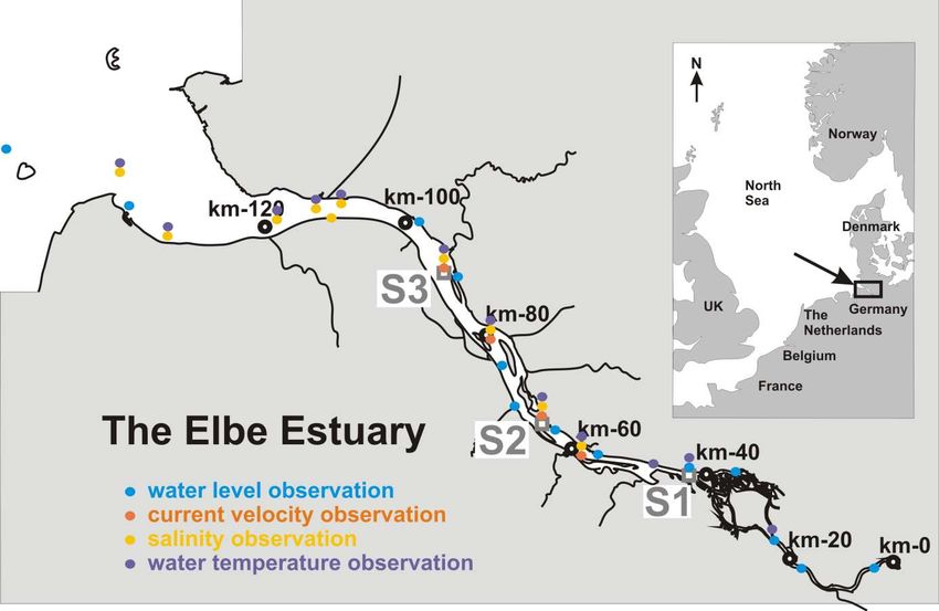
Die Küste, 87, 2019 https://doi.org/10.18171/1.087109

the ubiquity of bathymetric deepening, the influence of man-made bathymetric modifica-
tion on transport time has not been quantitatively investigated to date.
 Several methods exist to estimate time scales for the transport of substances. Some
methods provide an integral time scale for the entire system; others give local results for
the different positions in the estuary (Zimmerman 1988). The former kind of methods are
so-called box model estimates (Kärnä and Baptista 2016, Zimmerman 1988) which usually
either base on the flushing time approach (Monsen et al. 2002, Zimmerman 1988), make
use of particle tracking methods (Rayson et al. 2016) or rely on tidal prism models (Luketina
1998). Local time scales are either section-wise applications of the box model estimates, or
continuous methods that make use of numerical models. Of those local and continuous
methods, the concept of water age is a widely used method (Brye et al. 2012, Kärnä and
Baptista 2016, Shen and Haas 2004); it is mathematically well-described (Deleersnijder et
al. 2001, Delhez et al. 1999, Delhez et al. 2004, Delhez et al. 2014, Delhez and Deleersnijder
2002) and demarcated from related time scales (Delhez et al. 2014).

Figure 1: Location of the Elbe Estuary at the North Sea (small map). Thick black circles mark the
distance in kilometers downstream of the tidal barrier at km-0. The blue circles show the position
of the gauges (from upstream to downstream) Altengamme, Over, Bunthaus, Hamburg St. Pauli,
Seemannshoeft, Schulau, Hetlingen, Stadersand, Grauerort, Glueckstadt, Brokdorf, Cuxhaven, and
Scharhoern. The most downstream gauging station Bake Alpha lies outside of the map. The orange
circles show the position of the observation stations for current velocity (from upstream to down-
stream) D1 Hanskalbsand, D2 Julesand, D3 Pagensand, D4 Rhinplate. The yellow circles show the
position of the salinity observation stations (from upstream to downstream) D1 Hanskalbsand,
D2 Julesand, D3 Pagensand, D4 Rhinplate, LZ1a, LZ1, LZ1b, LZ2, LZ3 and LZ4. The violet
circles show the position of the water temperature observation stations (from upstream to down-
stream) Bunthaus, Seemannshoeft, Blankenese, D1 Hanskalbsand, D2 Julesand, D3 Pagensand,
D4 Rhinplate, LZ1a, LZ1b, LZ2, LZ3 and LZ4. The three grey squares mark the specific positions
S1, S2 and S3 for the analysis later on.

 263

Die Küste, 87, 2019 https://doi.org/10.18171/1.087109

In this study, we examine the effect of a realistic bathymetric change on transport time
scale. The bathymetric change reflects 40 years of human interference in the Elbe Estuary
(Germany), see Figure 1. According to the classification of Savenije (2005), the Elbe Estu-
ary is a funnel shaped alluvial estuary with an amplification of the tide in upstream direction.
In the estuarine parameter space of Geyer and MacCready (2014), the Elbe Estuary extends
from well-mixed to partially mixed conditions, depending on the position within the estu-
ary. The Elbe Estuary is strongly exposed to anthropogenic influences, particularly by
strong man-made modifications of its geometry with considerable deepening of the ba-
thymetry during the last centuries, but also by riverine substance loads which lead to strong
biogeochemical processes and the formation of a seasonal oxygen minimum zone in the
estuarine freshwater section (Amann et al. 2012, 2014, Bergemann et al. 1996, Dähnke et
al. 2008, Schöl et al. 2014, Schroeder 1997).

2 Method
2.1 Hydrodynamic model
We simulated hydrodynamics in the Elbe Estuary with the mathematical method Untrim
(Casulli 2009, Casulli and Stelling 2010). The Elbe Estuary model setup is adapted from the
coarsest model described in (Sehili et al. 2014). In comparison to the model used there, the
largest difference in the model applied here is the use of a detailed distribution of bottom
friction coefficients. The bathymetry resolution on subgrid level (Casulli and Stelling 2010)
enables a precise representation of water volume. The unstructured, orthogonal computa-
tional grid consists of roughly 11000 horizontal elements with 25 subgrid divisions per edge
and a maximum of 31 vertical z-layers with a thickness of 1m.
 The model domain extends along the 170 km estuarine shipping channel, starting at the
weir Geesthacht (km-0, see Figure 1) down to the end of the maintained shipping channel
in the inner German Bight, see Figure 2a. The domain contains the entire volume between
the main dikes and includes the largest eight tributaries of the estuary.
 The model is steered with realistic boundary values for the years 2010 and 2011: at the
riverine boundary, we use daily measurements of river discharge at the last riverine gauging
station Neu Darchau (50 km upstream of the weir at km-0; data from Water and Shipping
Authority Lauenburg, accessed at www.fgg-elbe.de). The highest discharge during the sim-
ulation period occurred at the end of January 2011 with a peak value of 3500 m3 s-1, and
long-lasting low discharge, ranging between 300–500 m3 s-1, was observed from May to end
of July 2011. Riverine water temperatures have a clear seasonal cycle with lowest values of
2–5°C at the beginning of the year, and highest values of 20–23°C during June to Septem-
ber. Riverine water temperatures originate from observations at the station Cumlosen
(115 km upstream of the weir at km-0; data from Landesamt für Umwelt Brandenburg,
accessed at www.fgg-elbe.de).
 The boundary value for salinity is kept constant at 0.4 psu. In the tributaries we employ
long-term mean discharge estimates (IKSE 2005) due to a lack of discharge measurements.
Wind and air temperature fields for the entire domain are provided with a spatial resolution
of 0.0625° (~ 7 km) from 24-hour-forecasts at 1 hour time resolution (Deutscher Wetter-
dienst DWD). At the seaward open boundary, water level values stem from a numerical
circulation model of the German Bight, the salinity value is kept constant at 32 psu and we

264

Die Küste, 87, 2019 https://doi.org/10.18171/1.087109

use water temperature values from the offshore observation station FINO1 (data from
http://fino.bsh.de) which is located outside the model domain in the North Sea.

2.2 Scenario definitions
Two different bathymetric scenarios represent two states with different degrees of man-
made modification: scenario “Hi” represents an actual, strongly impacted bathymetry. Sce-
nario “Lo” represents a lesser impacted bathymetry, though far from being pristine. The
modifications from Lo to Hi particularly include deepening and maintenance of the navi-
gation channel, and silting of flood plains and side branches as related morphological reac-
tions. Figure 2b and Figure 2c show that water depth in Hi is several meters larger com-
pared to Lo in most sections of the navigation channel.
 In Hi we use the bathymetry of the year 2010 as the most recent and consistent one
available. In Lo, we replace the bathymetry in the section between the tidal barrier and
km-120 by the 40 years older bathymetry of 1970. In the section of the replacement,
bathymetry differences can be mainly attributed to anthropogenic modifications. The ba-
thymetry of the estuarine mouth area further downstream was not changed in the model
since there, bathymetric differences mainly result from natural morphologic changes. Note
that the peculiar depth peak in scenario Lo at km-40 (Figure 2c) is due to the open con-
struction of an immersed tube tunnel below the Elbe at that time.
 We combine the two bathymetric scenarios Hi and Lo with four different discharge
regimes, resulting in eight simulated scenarios, see Table 1: Hi-M and Lo-M include the
variable, observed riverine freshwater discharge in the years 2010 and 2011. Hi-3 and
Lo-3 run with a constant discharge of 300 m3 s-1, corresponding to mean low summer
discharge of 301 m3 s-1 (FHH and HPA 2014). Hi-7 and Lo-7 (Hi-13 and Lo-13) run with
700 m3 s-1 (1300 m3 s-1), corresponding to mean discharge of 713 m3 s-1, and mean high
summer discharge of 1280 m3 s-1, respectively.
Table 1: Overview on scenarios; scenarios differ in bathymetry (Hi, Lo) and riverine freshwater
inflow. The reference simulation Hi-M is based on the bathymetry Hi and measured riverine dis-
charge; Hi-M thus represents the situation in the years 2010 and 2011.

Freshwater Measured Constant Constant Constant
discharge 2010 – 2011 300 m3 s-1 700 m3 s-1 1300 m3 s-1

Hi Hi-M (reference) Hi3 Hi7 Hi13

Lo Lo-M Lo3 Lo7 Lo13

 265

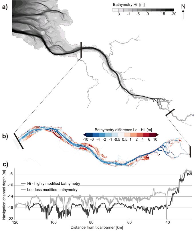
Die Küste, 87, 2019 https://doi.org/10.18171/1.087109

Figure 2: a) Model domain with bathymetry Hi, shown in the resolution as used in the subgrid
bathymetry model. Thick black lines mark the section of largest bathymetry differences between
Hi and Lo. b) Bathymetry difference Lo – Hi. Blue areas indicate that these parts are deeper
whereas red areas are lower in the bathymetry Hi. c) Depth of the navigation channel along the
estuary for the bathymetries Hi in black and Lo in grey.

266

Die Küste, 87, 2019 https://doi.org/10.18171/1.087109

2.3 Water age calculation
Delhez et al. (1999) defines the age of a water parcel as the time that elapsed since the water
parcel entered a domain of interest outside of which the age is prescribed to be zero.
Thereby, age is a pointwise, time-dependent result in the domain and its calculation is de-
rived in an Eulerian framework to run with the algorithms of a numerical model.
 We use the calculation of water age implemented in D-Water Quality (Postma et al.
2003, Smits and van Beek 2013), which is based on the tracking of two tracers that are
transported by fluid motion. One tracer (Tcon) is conservative whereas the other tracer
(Tdec) is subjected to exponential growth or decay and related to the concentration of Tcon
according to: ( ) = ∙ − .
 The transport equations for the two tracers are
 
 = −∇ ∙ ( − ∇ ) (1)
 
 = − − ∇ ∙ ( − ∇ ) (2)
 
The water age a is then calculated by
 ln( ⁄ )
 = (3)
 − 

We focus on the age of riverine water because the riverine substance load governs the
strong biogeochemical processes in the Elbe Estuary (Amann et al. 2012, 2012, 2014, 2014,
Dähnke et al. 2008, Schroeder 1997). To estimate the time that elapsed since a riverine
water signal entered the estuary, we charge water discharge at the tidal barrier with constant
concentrations of the conservative as well as the decayable tracer. The decay rate of the
decayable tracer is chosen to be γ=0.01 [d-1]. During the simulation, riverine water age ariv
is then calculated for each computational element, based on Equation 3.

2.4 Calculation of hydraulic residence time
The hydraulic residence time tres (Monsen et al. 2002; Zimmerman 1988), is defined as
 = ∙ −1 , (4)
where V is the estuarine volume upstream of a specific position, and Q is freshwater dis-
charge. The definition of hydraulic residence time tres in Equation (4) assumes stationary
discharge and a completely mixed water volume.
 Here, we determined tres for the constant discharge scenarios Hi3, Hi7, and Hi13 by
using the results of the hydrodynamic simulation for the calculation of V. We proceeded
as follows: starting at the upstream model boundary (river boundary), we specified posi-
tions and corresponding cross sections every two kilometres downstream of each other.
Solely the area where the estuary forms an inland delta and splits into a southern and north-
ern stream, between km-22 and km-40, was not subdivided into smaller sections. The last
cross section is located at km-114, where the estuarine funnel starts to open to the sea and
extensive tidal flats are present. For each position, we calculated the upstream estuarine
water volumes by summing up the water volumes of all computational cells located

 267

Die Küste, 87, 2019 https://doi.org/10.18171/1.087109

upstream of the corresponding cross section. Finally, we averaged these aggregated water
volumes over a spring-neap cycle.
 This section-wise information on the average water volume for each constant discharge
scenario was then used to calculate tres along the estuary.

3 Results
3.1 Hydrodynamic model validity
Reference simulation (Hi-M) results demonstrate that the hydrodynamic model is capable
of simulating the estuarine water movement with a good overall agreement between simu-
lated cell values and point measurements. The skill for a direct comparison of simulated
and observed values for water level, current velocity, salinity and water temperature is given
in Table 2 and Figure 3. For the skill assessment of water level, we used data from 14
observation stations, which were provided by the German Water and Shipping Administra-
tion. From upstream to downstream, these are the stations Altengamme, Over, Bunthaus,
Hamburg St. Pauli, Seemannshoeft, Schulau, Hetlingen, Stadersand, Grauerort, Glueck-
stadt, Brokdorf, Cuxhaven, Scharhoern and Bake A. For the skill assessment of current
velocity, salinity and water temperature, we compared depth averaged model results to the
observational values. For the stations D1 Hanskalbsand, D2 Julesand, D3 Pagensand, D4
Rhinplate (Water and Shipping Administration), which are equipped with a fixed bottom
sensor and a vertically moving top sensor 0.8 m below the water surface, observational
values were also depth averaged. In addition to these four stations, the stations LZ1a, LZ1,
LZ1b, LZ2, LZ3 and LZ4 (Water and Shipping Administration) were included in the skill
assessment for salinity and water temperature, and Bunthaus, Seemannshoeft and
Blankenese (Institut fuer Hygiene und Umwelt Hamburg, www.wgmn.hamburg.de, license
dl-de/by-2-0) for water temperature. Refer to Figure 1 for the positions of all observation
stations.
Table 2: Model skill in comparison to observations. n gives the number of observation stations.
The statistical figures were calculated using all available measurements at each station for the entire
simulation period from 01.01.2010 to 31.12.2011.

Variable with Root mean square
 Mean correlation Mean difference
n = number of stations error
Water level (n=14) 0.99 0.10 (m) 0.15 (m)
Current velocity (n=4) 0.930 0.11 (m/s) 0.12 (m/s)
Salinity (n=10) 0.867 2.10 (psu) 2.4 (psu)
Water temperature (n=12) 0.991 0.97 (°C) 1.23 (°C)

268

Die Küste, 87, 2019 https://doi.org/10.18171/1.087109

Figure 3: Normalized Taylor diagram on the statistical comparison of model results for the refer-
ence scenario Hi-M to observations. Blue dots show values for model skill at the positions of water
level measurements, red dots for current velocities, yellow dots for salinity and violet dots for water
temperature. Observation stations and period of comparison are identical to the ones assessed in
Table 2.

Time series comparison generally shows a good agreement between simulated and ob-
served water level and current velocity, including magnitude and timing, see two examples
in Figure 4 with a) at a position in the beginning of the salinity gradient zone, and b) at a
position in the freshwater zone, i.e. the section of the estuary where salinity is only deter-
mined by riverine salinity. However, the main shortcoming of the model is the intrusion of
salinity too far upstream, as can be seen in Figure 4 a): at the upstream end of the salt
mixing zone, the model overestimates salinity with 2 to 3 psu. The salinity stations which
show the noticeable poor skill in Figure 3 are located in this region. The deviation in water
temperature predominantly occurs during summer and mainly originates from neglecting
the effect of power plant cooling waters.
 The differences in tidal characteristic numbers of water level, see Table 3, show that
overall, the tidal curve is modeled with an 18 cm too large tidal range, which is almost
equally distributed between an overestimated high water level and an underestimated low
water level. High water and low water occur roughly 10 minutes later in the simulation,
while differences in the duration of flood period and ebb period are below one minute.
Our results complement (Sehili et al. 2014) who already showed good agreement between
model results and observations for water level during selected periods in the years 2006
and 2011. Altogether, the model provides a reliable hydrodynamic base.

 269

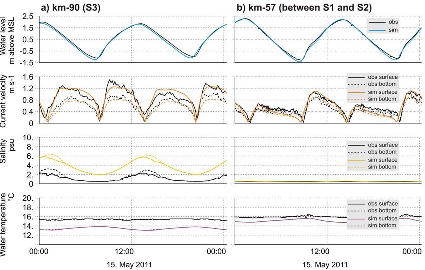
Die Küste, 87, 2019 https://doi.org/10.18171/1.087109

Figure 4: Time series comparison of observed and simulated water level, current velocity, salinity
and water temperature; a) at position km-90 with water level measured at Glueckstadt, and current
velocity, salinity and water temperature measured at D4 Rhinplate; b) at position km-57 with water
level measured at Schulau, and current velocity, salinity and water temperature measured at D1
Hanskalbsand.
Table 3: Differences in tidal characteristic numbers of water level between simulated results and
observational data (sim – obs) for the period 01.02.2010 to 31.12.2011, including 1349 tidal cycles
at 14 observation stations. Second column contains the mean difference over all stations, with the
mean values of absolute differences given in brackets. We used the postprocessors ncanalyse and
ncdelta for the analysis (http://wiki.baw.de/en/index.php/NCANALYSE and
http://wiki.baw.de/en/index.php/NCDELTA).
Difference in Mean (abs(mean)) Min Max

Mean high water level [m] + 0.09 (0.11) - 0.01 (Cuxhaven) + 0.21 (Bunthaus)

Mean low water level [m] - 0.09 (0.10) - 0.02 (Cuxhaven) - 0.19 (Altengamme)

Mean tidal range [m] + 0.18 (0.19) + 0.01 (Bake A) + 0.37 (Altengamme)

Mean water level [m] + 0.01 (0.03) - 0.07 (Bake A) + 0.06 (Hetlingen)

Time of high water [min] + 12.0 (12.3) -1 (Cuxhaven) + 20 (Grauerort)

Time of low water [min] + 7.8 (8.8) -6 (Cuxhaven) + 21 (Altengamme)

Flood period duration [min] - 0.5 (3.5) -15 (Altengamme) +6 (Grauerort)

Ebb period duration [min] + 0.3 (3.8) -5 (Grauerort) + 16 (Altengamme)

Flood mean water level [m] - 0.03 (0.04) - 0.08 (Grauerort) + 0.01 (Altengamme)

Ebb mean water level [m] + 0.04 (0.06) - 0.09 (Bake A) + 0.11 (Hetlingen)

270

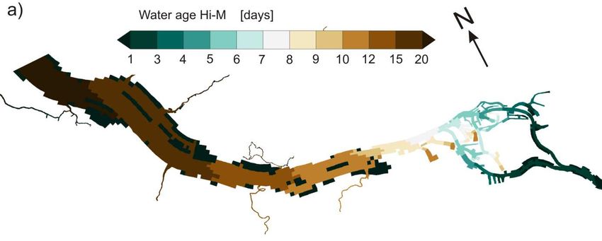
Die Küste, 87, 2019 https://doi.org/10.18171/1.087109

3.2 Reference water age
In the reference scenario Hi-M, riverine water age ariv generally increases from upstream to
downstream: Figure 5a shows ariv during the year 2011 at three stations S1, S2, S3 along the
estuarine shipping channel (positions marked in Figure 1) with S1 being the most upstream
station and having smaller ariv values than S2 than S3. The areal overview confirms that ariv
increases downstream, see Figure 6a, which shows spring-neap averaged ariv values during
low river discharge condition.
 Riverine water age ariv exhibits a strong dependency on river discharge (blue line in
Figure 5a): after the high discharge event at the end of January, ariv values are smallest for
all stations (e.g. 0.9 days at S1, 3.8 days at S3) while values are largest in July after several
weeks of low discharge (e.g. 9.1 days at S1, 25.2 days at S3). The further downstream the
station, the bigger is the difference between smallest ariv after high discharge and largest ariv
during low discharge: while this difference is about 8 days at S1, it is more than 20 days at
S3. The ariv difference between the stations also depends on discharge, e.g. the ariv differ-
ence between S1 and S3 after the peak discharge in January is about 3 days whereas it is
more than 15 days during the low flow period in June/July.
 When looking at ariv values in dependence on river discharge without chronological
allocation (dots in Figure 5b), the behavior described above appears even more consistent:
at similar discharge, ariv values are larger the further downstream the station; at the same
station, ariv values are larger the smaller the discharge; the further downstream the station,
the larger the ariv difference at high discharge compared to low discharge; and, finally, the
lower the discharge, the higher the ariv differences between upstream and downstream sta-
tions.
 At each station, ariv seems to be inversely proportional to river discharge Q; Figure 5b
displays a fitted line at each station S1 to S3 of ariv in dependence of Q-1.

Figure 5: a) Time series of measured river discharge Q (blue line) and calculated, tidally averaged
riverine water age ariv for the year 2011. Values for ariv are shown at the stations S1 (km-43, position
Seemannshöft) and S2 (km-65, D2 Julesand) in the estuarine freshwater part, and S3 (km-90, po-
sition D4 Rhinplate) in the salinity mixing zone for the scenarios Hi-M (black) and Lo-M (grey),
respectively. b) Black dots show daily ariv values plotted versus freshwater discharge Q for the
stations S1, S2 and S3; the lines show a fit for each station with the equation given in the box.

 271

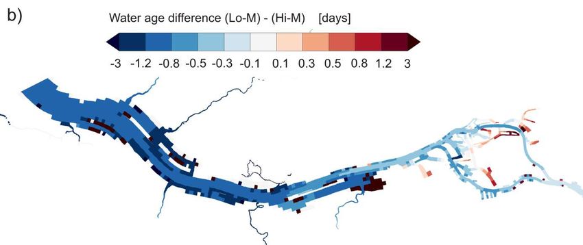
Die Küste, 87, 2019 https://doi.org/10.18171/1.087109

3.3 Water age for bathymetric and constant discharge scenarios
In scenario Lo-M, ariv is usually smaller compared to Hi-M, see in Figure 5a grey lines
compared to black lines. The differences are in the order of hours at S1, S2, and S3, and
thus lower than the differences caused by the natural variability of river discharge. At S1,
the difference in ariv between the two scenarios Hi-M and Lo-M is smallest following the
flood event (~ 1 hour difference) and highest during the low-flow period (~ 14 hours
difference). At S3, differences are larger but behave in the same way: differences are small-
est after the flood in January (~ 8 hours difference) and they are highest during low river
discharge (~ 38 hours).

Figure 6: a) Spring-neap tidally averaged water age ariv in June 2011 for scenario Hi-M. There are
some conspicuous patches in the middle of the estuary (sand banks and islands) and at the banks
that appear to have a water age below 1 day: these are elevated areas that have fallen dry and have
a water age of zero. b) Water age difference (Lo-M) – (Hi-M) of spring-neap tidally averaged water
age for boundary conditions of June 2011. Similar to a), there are patches where water age differ-
ence above 3 days is displayed: these areas fell dry in Hi-M but not in Lo-M, leading to the appar-
ently high difference.

The areal differences between Hi-M and Lo-M (Figure 6b) confirm that ariv is larger in
Hi-M, apart from some harbor basins and bank areas that silted up or had been backfilled.
Figure 6b also indicates that ariv differences increase downstream.

272

Die Küste, 87, 2019 https://doi.org/10.18171/1.087109

 In the constant freshwater discharge scenarios (Hi3, Hi7, Hi13), riverine water age ariv
behaves similarly to the scenarios with variable, measured discharge: ariv increases with dis-
tance from the tidal barrier and with decreasing discharge (Figure 7 upper left panel). In
addition to the variable discharge scenarios, the quasi-stationary results for the constant
discharge scenarios better allow an evaluation on the longitudinal profile. Most prominent
is the accelerated increase in ariv between km-20 and km-35 (Figure 7 zoom area on upper
right panel). During the 15 km long distance, ariv increases from 1.5 days to 6.4 days in the
low-flow scenario Hi3, from 14 hours to 2.5 days in Hi7 and from 8 hours to 1.3 days in
Hi13. Downstream of km-35, the increase in ariv continues steadily but more gradually.
55 km further downstream, at position S3, ariv reaches values of 24.8 days in Hi3, of 15.6
days in Hi7 and of 9.5 days in Hi13.
 Water age in the corresponding Lo constant discharge scenarios is always smaller (Fig-
ure 7 upper panels, flat-colored lines for Lo-scenarios in comparison to intensely-colored
lines for Hi-scenarios). However, differences are in the order of a few hours up to 1 day
maximum (see Figure 7 lower panels). While ariv differences between Hi7 and Lo7, and
Hi13 and Lo13, grow almost continuously from upstream to downstream until km-70 in
Lo7 and until km-100 in Lo13, the differences between Hi3 and Lo3 peak twice along the
estuary: at around km-30 where ariv is 16 hours smaller, and second between km-60 and
km-80 where it is almost 1 day smaller in the shallower bathymetry Lo. Downstream of
km-80, ariv values in Hi3 and Lo3 converge whereas differences in Hi7/Lo7, Hi13/Lo13
respectively, appear to remain almost constant until km-140.

Figure 7: Upper panels: Riverine water age along the estuary for scenarios with constant discharge.
Lower panels: Difference in riverine water age between scenarios with the same discharge but
different bathymetries. Left panels show values along the entire shipping channel, right panels
show a zoom in the upstream 40 km of the shipping channel.

 273

Die Küste, 87, 2019 https://doi.org/10.18171/1.087109

4 Discussion
4.1 Relation between water age and river discharge
Riverine water age ariv is determined by river discharge (Figure 5). The dependency between
ariv and Q is clearest at the most upstream position S1 and, because of a delayed response,
becomes less distinct further downstream: the effect of a change in Q needs some time to
propagate through the system and the assumption of fast/instantaneous adaptation of ariv
becomes less precise the more downstream the location of interest. This delayed response
also causes the difference at high discharge values between ariv and the fitted line in Figure
5 b), which is particularly evident for the position S3. A possibility for a better fit was to
relate the riverine water age ariv(x,t) at an arbitrary position x downstream of the discharge
(x = 0) and at an arbitrary point in time t to the entire discharge history between t- ariv(x,t)
and t. However, the capability to predict ariv would be lost by using such a relationship.
 The observed inverse proportionality between ariv and Q (Figure 5 b) can be explained
by the hydraulic residence time tres: Figure 8 shows both transport time scales, ariv and tres,
for the constant discharge scenarios on the actual, strongly impacted bathymetry. For each
discharge scenario, the two transport time scales are similar in the freshwater region. The
differences are in the range of hours between the hydraulic residence time tres, which con-
stitutes an integral measure for the entire water volume upstream of a specific position, and
riverine water age ariv, which gives a local value. Their similarity illustrates the well-mixed
nature of the freshwater zone and demonstrates that ariv is mainly driven by downstream-
oriented residual flow which is induced by discharge.
 It has to be noted that the limit of the freshwater region depends on discharge and
migrates upstream with decreasing discharge. The model simulates the freshwater limit at
around km-55 for a constantly low discharge of 300 m3 s-1 (in Scenario Hi3), at km-85 in
Hi7, and at km-105 in Hi13. However, the salt front in the model penetrates too far land-
wards, see Figure 4, so the above given limits of the freshwater region can be expected to
be located several kilometres further downstream.
 Downstream of the freshwater region, the two transport time scales increasingly deviate
from each other, mainly because of two reasons: first and foremost, the volume V in Equa-
tion (4) is progressively filled with seawater instead of water that originates from river dis-
charge. Second, the underlying assumption in Equation (4) of a completely mixed water
volume becomes continuously less valid with downstream position.
 In contrast to tres, ariv remains a valid transport time scale for river water throughout the
estuary because it gives the time that has elapsed since the water entered the estuary at the
upstream boundary, independent of the ratio of freshwater to seawater and under varying
discharge.
 So far, the concept of water age has mainly been applied in systems characterized by
stratification, and a strong dependency of water age on discharge has also been found in
these systems. There, in addition to a general decrease in water age with increasing dis-
charge, an influence is also given by a larger vertical difference between smaller age values
at the surface and larger age values at the bottom (Kärnä and Baptista 2016, Ren et al. 2014,
Shen and Lin 2006). Apart from discharge, tidal forcing (Shen and Lin 2006) and wind
(Gong et al. 2009) have been described to influence the vertical distribution of age in strat-
ified systems.

274

Die Küste, 87, 2019 https://doi.org/10.18171/1.087109

Figure 8: Riverine water age (solid lines) and hydraulic residence times (dots) for the constant
discharge scenarios Hi3 (green), Hi7 (blue) and Hi13 (red) along the shipping channel. The gap in
hydraulic residence time data between km-22 and km-40 is because the inland delta in that area has
not been divided into separate sections for the analysis of water volume.

4.2 Effect of man-made bathymetric modification on water age
The variation in water age ariv due to varying discharge within each of the scenarios Hi-M
and Lo-M is much larger than the difference in ariv due to a different bathymetry at any
equal discharge regime, although large depth differences exist between the bathymetric sce-
narios Hi and Lo (Figure 2b and Figure 2c). In scenario Hi, the navigation channel is several
meters deeper whereas lateral areas at the banks of the estuary are up to several meters
shallower. In total, the estuarine volume is about 6.7 % larger in Hi compared to Lo. The
larger water volume explains the general increase in riverine water age under the higher
human impact in Hi-M.
 During the time period that we considered in this study, discharge values were not con-
stant long enough for ariv to reach steady state values. We therefore also studied scenarios
with different constant discharges and found the ariv differences between the bathymetric
scenarios (Hi3 and Lo3, Hi7 and Lo7, Hi13 and Lo13, respectively) to be in the same order
of magnitude as the difference between Hi-M and Lo-M. This consistency in results for
different discharge regimes lets us reliably determine the difference in ariv due to the bath-
ymetric modifications to be in the order of several hours in most sections of the estuary,
corresponding to 6–8 % of the absolute value. This relative increase in riverine water age
in the higher impacted bathymetry corresponds to the relative increase in water volume.
Thus, the difference in riverine water age can also be explained quantitatively by the in-
crease in volume, considering the similarity to hydraulic residence time: in Equation (4), a
variation in volume directly changes tres by the same relative amount.
 This almost direct quantitative dependency between a change in water volume and a
change in age can be expected to be generally applicable to well-mixed estuaries, or well-
mixed sections of otherwise more stratified estuaries. In contrast, in stratified estuaries,

 275

Die Küste, 87, 2019 https://doi.org/10.18171/1.087109

where a vertical variability in age and other additional influences apart from discharge on
the vertical age distribution play a role, a more complex relation may exist.

4.3 Relation to estuarine oxygen dynamics
Transport time scales are usually explored in the context of biogeochemical or water quality
issues (Ahmed et al. 2017, Brye et al. 2012, Chan et al. 2002, Fujiwara et al. 2002, Rayson
et al. 2016, Shen and Haas 2004). Here, we focus on estuarine oxygen dynamics because in
the Elbe Estuary (Amann et al. 2012, Schroeder 1997) and in many other contemporary
estuaries worldwide, estuarine oxygen minimum zones (eOMZs) are frequently observed
(Abril et al. 2003, Billen et al. 2001, Hagy et al. 2004, Ruiz et al. 2015, Tomaso and Najjar
2015, Zhang and Li 2010). The eOMZs are mainly linked to anthropogenic impacts, of
which eutrophication is the most frequently reported cause (Breitburg et al. 2003, Cloern
2001, Conley et al. 2009, Diaz 2001, Díaz and Rosenberg 2011, Howarth et al. 2011, Kemp
et al. 2009, Paerl 2006, 2009, Rabalais et al. 2010): the increase in land-borne nutrients due
to the wash out of agricultural fertilizers increases primary production in the limnic river
sections which transforms into labile detritus when reaching the deeper and more turbid
estuarine sections. Bacterial respiration of such easily degradable detritus consumes oxygen
and results in an eOMZ if the oxygen depletion cannot be counterbalanced by atmospheric
reaeration or primary production.
 Generally, physical and biogeochemical processes interact in the formation and control
of eOMZs (Du and Shen 2015, Kemp and Boynton 1980). Previous studies have attempted
to estimate the effect of physical processes on eOMZs, mainly for stratified and partially
stratified estuaries (Bruce et al. 2014, Du and Shen 2015, Fujiwara et al. 2002, Scully 2013),
where wind conditions and freshwater discharge govern the strength of the stratification
and thus are the dominating physical influence mechanisms.For well-mixed estuaries, com-
parable studies are missing, maybe because the intrinsic hydrodynamic conditions are fa-
vourable to counteract low dissolved oxygen concentrations by the generally greater possi-
bility to supply oxygenated water from the surface. Nevertheless, eOMZs regularly occur
in many well-mixed estuaries (Diez-Minguito et al. 2014, Lanoux et al. 2013, Schroeder
1997, Verity et al. 2006).
 Bathymetric deepening in well-mixed estuaries influences physical factors of eOMZ
formation, mainly the transport of degradable organic matter via changes in hydrodynamics
and the relative atmospheric interface for reaeration due to the reduction in water surface-
to-volume ratio. Despite these possible influences of bathymetric deepening on an eOMZ,
there is no quantification of physical effects known to us, though, similar to the Elbe Es-
tuary, many well-mixed estuaries worldwide experience the phenomena of a strongly deep-
ened navigation channel and severe eOMZs, like the upper Delaware Estuary (DiLorenzo
et al. 1994, Sharp 2010, Tomaso and Najjar 2015), the Scheldt (Meire et al. 2005, van
Damme et al. 2005), the Loire (Abril et al. 2003, Etcheber et al. 2007, Walther et al. 2015)
or the Guadalquivir (Diez-Minguito et al. 2014, Ruiz et al. 2015).
 The time it takes for degradable organic matter to be transported to a specific location
determines the completeness of its heterotrophic degradation. Middelburg and Herman
(2007), for example, showed that organic matter is extensively modified due to hetero-
trophic processing in estuaries with long residence times compared to estuaries with shorter
residence times. An analysis in Lanoux et al. (2013) for the Gironde estuary hints at lower

276

Die Küste, 87, 2019 https://doi.org/10.18171/1.087109

oxygen concentration during a period of longer residence times compared to a period of
shorter residence time under otherwise similar environmental conditions. It is thus a plau-
sible concept that a longer transport time induces higher accumulated oxygen consumption
between the origin of degradable organic matter and some specific location.
 Given the detected increase in ariv of approximately 7 %, our results hint at an increase
in accumulated oxygen demand caused by a realistic, 40-year bathymetric change due to
human interference. If the higher oxygen consumption will also finally lead to a more se-
vere eOMZ, strongly depends on the possibility for reaeration (Holzwarth and Wirtz 2018).

5 Conclusion
This is the first study on the impact of a bathymetry difference on riverine transport time
scale in an estuary. We show for the Elbe Estuary that the effect of a bathymetric differ-
ence, which reflects a realistic 40-year impact of typical man-made modification, on riverine
water age is much smaller than the effect of the natural, seasonal variability in river dis-
charge. The age difference between the bathymetric scenarios lies in the order of hours up
to one day maximum, depending on location and discharge. This difference corresponds
to a 6–8 % larger relative riverine water age in the bathymetry with higher human impact.
 Due to the well-mixed character of the Elbe Estuary, this increase in riverine water age
is mainly caused by the increase in water volume, and an almost direct quantitative depend-
ency between a change in water volume and a change in age exists.
 Generally, riverine water age in the Elbe Estuary is governed by river discharge; the age
is small after time intervals with high discharges and increases, proportional to the inverse
of discharge, during periods of low discharge. Thereby, the age difference between highest
and lowest discharge is in the order of days for upstream stations and grows to weeks for
stations in the salinity gradient zone.
 Notwithstanding the apparently small impact, the effect of the larger water age in the
higher impacted bathymetry potentially leads to higher accumulated oxygen consumption.
In combination with reduced oxygen reaeration due to the decreased water surface-to-vol-
ume ratio, the higher impacted bathymetry generates additional stressors to the estuarine
oxygen minimum zone, acting into the direction of lower oxygen levels. We thus expect
hydrodynamic effects by bathymetry deepening to intensify the eutrophication impact on
estuarine oxygen levels.

6 Acknowledgements
We thank Frank Böker (BAW) for preparing the different model bathymetries and Günther
Lang (BAW) for his valuable input on the hydrodynamic simulations and the postpro-
cessing of the results.
 The work of Ingrid Holzwarth and Holger Weilbeer was funded as part of the Federal
Waterways Engineering and Research Institute (BAW) departmental research and develop-
ment program. The work of Kai W. Wirtz was supported by the German Federal Ministry
of Education and Research (BMBF) through the MOSSCO project and by the Helmholtz
Society through the PACES program.

 277

Die Küste, 87, 2019 https://doi.org/10.18171/1.087109

7 References
Abood, K. A.; Metzger, S. G.; Distante, D. F.: Minimizing Dredging Disposal via Sediment
Management in New York Harbor. In: Estuaries, 22, 3, 763, 1999.
Abril, G.; Etcheber, H.; Delille, B.; Frankignoulle, M.; Borges, A. V.: Carbonate dissolution
in the turbid and eutrophic Loire estuary. In: Marine Ecology Progress Series, 259, 129–
138, 2003.
Ahmed, A.; Pelletier, G.; Roberts, M.: South Puget Sound flushing times and residual flows.
In: Estuarine, Coastal and Shelf Science, 187, 9–21, 2017.
Amann, T.; Weiss, A.; Hartmann, J.: Carbon dynamics in the freshwater part of the Elbe
estuary, Germany: Implications of improving water quality. In: Estuarine, Coastal and Shelf
Science, 107, 112–121, 2012.
Amann, T.; Weiss, A.; Hartmann, J.: Silica fluxes in the inner Elbe Estuary, Germany. In:
Biogeochemistry, 118, 1–3, 389–412, 2014.
Avoine, J.; Allen, G. P.; Nichols, M.; Salomon, J. C.; Larsonneur, C.: Suspended-sediment
transport in the Seine estuary, France. Effect of man-made modifications on estuary-shelf
sedimentology. In: Marine Geology, 40, 1–2, 119–137, 1981.
Bergemann, M.; Blöcker, G.; Harms, H.; Kerner, M.; Meyer-Niehls, R.; Petersen, W.;
Schroeder, F.: Der Sauerstoffhaushalt der Tideelbe. In: Die Küste, 58, 199–261, 1996.
Billen, G.; Garnier, J.; Ficht, A.; Cun, C.: Modeling the response of water quality in the
Seine River Estuary to human activity in its watershed over the last 50 years. In: Estuaries,
24, 6, 977, 2001.
Breitburg, D. L.; Adamack, A.; Rose, K. A.; Kolesar, S. E.; Decker, B.; Purcell, J. E.; Keister,
J. E.; Cowan, J. H.: The pattern and influence of low dissolved oxygen in the Patuxent
River, a seasonally hypoxic estuary. In: Estuaries, 26, 2, 280–297, 2003.
Bruce, L. C.; Cook, P. L. M.; Teakle, I.; Hipsey, M. R.: Hydrodynamic controls on oxygen
dynamics in a riverine salt wedge estuary, the Yarra River estuary, Australia. In: Hydrology
and Earth System Sciences, 18, 4, 1397–1411, 2014.
Brye, B. de; Brauwere, A. de; Gourgue, O.; Delhez, E. J.M.; Deleersnijder, E.: Water re-
newal timescales in the Scheldt Estuary. In: Journal of Marine Systems, 94, 74–86, 2012.
Casulli, V.: A high-resolution wetting and drying algorithm for free-surface hydrodynamics.
In: International Journal for Numerical Methods in Fluids, 60, 4, 391–408, 2009.
Casulli, V.; Stelling, G. S.: Semi-implicit subgrid modelling of three-dimensional free-sur-
face flows. In: International Journal for Numerical Methods in Fluids, 67, 4, 441–449, 2010.
Chan, T. U.; Hamilton, D. P.; Robson, B. J.; Hodges, B. R.; Dallimore, C.: Impacts of
hydrological changes on phytoplankton succession in the Swan River, Western Australia.
In: Estuaries, 25, 6, 1406–1415, 2002.
Cloern, J. E.: Our evolving conceptual model of the coastal eutrophication problem. In:
Marine Ecology Progress Series, 210, 223–253, 2001.

278

Die Küste, 87, 2019 https://doi.org/10.18171/1.087109

Conley, D. J.; Paerl, H. W.; Howarth, R. W.; Boesch, D. F.; Seitzinger, S. P.; Havens, K. E.;
Lancelot, C.; Likens, G. E.: Ecology. Controlling eutrophication. Nitrogen and phospho-
rus. In: Science (New York, N.Y.), 323, 5917, 1014–1015, 2009.
Dähnke, K.; Bahlmann, E.; Emeis, K.: A nitrate sink in estuaries? An assessment by means
of stable nitrate isotopes in the Elbe estuary. In: Limnology and Oceanography, 53, 4,
1504–1511, 2008.
Deleersnijder, E.; Campin, J.-M.; Delhez, E. J. M.: The concept of age in marine modelling.
In: Journal of Marine Systems, 28, 3–4, 229–267, 2001.
Delhez, E. J.M.; Campin, J.-M.; Hirst, A. C.; Deleersnijder, E.: Toward a general theory of
the age in ocean modelling. In: Ocean Modelling, 1, 1, 17–27, 1999.
Delhez, É. J.M.; Brye, B. de; Brauwere, A. de; Deleersnijder, É.: Residence time vs influence
time. In: Journal of Marine Systems, 132, 185–195, 2014.
Delhez, É. J.M.; Deleersnijder, É.: The concept of age in marine modelling. In: Journal of
Marine Systems, 31, 4, 279–297, 2002.
Delhez, É. J.M.; Lacroix, G.; Deleersnijder, É.: The age as a diagnostic of the dynamics of
marine ecosystem models. In: Ocean Dynamics, 54, 2, 221–231, 2004.
Díaz, R. J.: Overview of hypoxia around the world. In: Journal of Environment Quality,
30, 2, 275, 2001.
Díaz, R. J.; Rosenberg, R.: Introduction to Environmental and Economic Consequences
of Hypoxia. In: International Journal of Water Resources Development, 27, 1, 71–82, 2011.
Diez-Minguito, M.; Baquerizo, A.; Swart, H. E. de; Losada, M. A.: Structure of the turbidity
field in the Guadalquivir estuary. Analysis of observations and a box model approach. In:
Journal of Geophysical Research: Oceans, 119, 10, 7190–7204, 2014.
DiLorenzo, J. L.; Huang, P.; Thatcher, M. L.; Najarian, T. O.: Dredging Impacts on Dela-
ware Estuary Tides. In: Spaulding, M. L. (ed.): Proceedings of the 3rd international confer-
ence / 3rd International Conference on Estuarine and Coastal Modeling. Oak Brook, Illi-
nois, September 8–10, 1993, American Soc. of Civil Engineers, New York, NY, 1994.
Du, J.; Shen, J.: Decoupling the influence of biological and physical processes on the dis-
solved oxygen in the Chesapeake Bay. In: Journal of Geophysical Research: Oceans, 120,
1, 78–93, 2015.
Ensing, E.; Swart, H. E. de; Schuttelaars, H. M.: Sensitivity of tidal motion in well-mixed
estuaries to cross-sectional shape, deepening, and sea level rise. In: Ocean Dynamics, 65,
7, 933–950, 2015.
Etcheber, H.; Taillez, A.; Abril, G.; Garnier, J.; Servais, P.; Moatar, F.; Commarieu, M.-V.:
Particulate organic carbon in the estuarine turbidity maxima of the Gironde, Loire and
Seine estuaries: Origin and lability. In: Hydrobiologia, 588, 1, 245–259, 2007.
FHH; HPA: Deutsches gewässerkundliches Jahrbuch. Elbegebiet, Teil III: Untere Elbe ab
der Havelmündung. In German, Hamburg, 2014.

 279

Die Küste, 87, 2019 https://doi.org/10.18171/1.087109

Fujiwara, T.; Takahashi, T.; Kasai, A.; Sugiyama, Y.; Kuno, M.: The role of circulation in
the development of hypoxia in Ise Bay, Japan. In: Estuarine, Coastal and Shelf Science, 54,
1, 19–31, 2002.
Geyer, W. R.; MacCready, P.: The Estuarine Circulation. In: Annual Review of Fluid Me-
chanics, 46, 1, 175–197, 2014.
Gong, W.; Shen, J.; Hong, B.: The influence of wind on the water age in the tidal Rappa-
hannock River. In: Marine Environmental Research, 68, 4, 203–216, 2009.
Hagy, J. D.; Boynton, W. R.; Keefe, C. W.; Wood, K. V.: Hypoxia in Chesapeake Bay,
1950–2001. Long-term change in relation to nutrient loading and river flow. In: Estuaries,
27, 4, 634–658, 2004.
Holzwarth, I.; Wirtz, K.: Anthropogenic impacts on estuarine oxygen dynamics. A model
based evaluation. In: Estuarine, Coastal and Shelf Science, 211, 45–61, 2018.
Howarth, R.; Chan, F.; Conley, D. J.; Garnier, J.; Doney, S. C.; Marino, R.; Billen, G.: Cou-
pled biogeochemical cycles. Eutrophication and hypoxia in temperate estuaries and coastal
marine ecosystems. In: Frontiers in Ecology and the Environment, 9, 1, 18–26, 2011.
IKSE: Die Elbe und ihr Einzugsgebiet. Ein geographisch-hydrologischer und wasserwirt-
schaftlicher Überblick. In German, International Commission for the Protection of the
Elbe, Magdeburg, 2005.
Kärnä, T.; Baptista, A. M.: Water age in the Columbia River estuary. In: Estuarine, Coastal
and Shelf Science, 183, 249–259, 2016.
Kemp, W. M.; Boynton, W. R.: Influence of biological and physical processes on dissolved
oxygen dynamics in an estuarine system. Implications for measurement of community me-
tabolism. In: Estuarine and Coastal Marine Science, 11, 4, 407–431, 1980.
Kemp, W. M.; Testa, J. M.; Conley, D. J.; Gilbert, D.; Hagy, J. D.: Temporal responses of
coastal hypoxia to nutrient loading and physical controls. In: Biogeosciences, 6, 12, 2985–
3008, 2009.
Lane, A.: Bathymetric evolution of the Mersey Estuary, UK, 1906–1997. Causes and ef-
fects. In: Estuarine, Coastal and Shelf Science, 59, 2, 249–263, 2004.
Lanoux, A.; Etcheber, H.; Schmidt, S.; Sottolichio, A.; Chabaud, G.; Richard, M.; Abril, G.:
Factors contributing to hypoxia in a highly turbid, macrotidal estuary (the Gironde, France).
In: Environmental Science: Processes & Impacts, 15, 3, 585, 2013.
Liu, W.-C.; Hsu, M.-H.; Kuo, A. Y.; Li, M.-H.: Influence of bathymetric changes on hydro-
dynamics and salt intrusion in estuarine system. In: Journal of the American Water Re-
sources Association, 37, 5, 1405–1416, 2001.
Luketina, D.: Simple Tidal Prism Models Revisited. In: Estuarine, Coastal and Shelf Sci-
ence, 46, 1, 77–84, 1998.
Meire, P.; Ysebaert, T.; van Damme, S.; van den Bergh, E.; Maris, T.; Struyf, E.: The Scheldt
estuary. A description of a changing ecosystem. In: Hydrobiologia, 540, 1–3, 1–11, 2005.
Meyers, S. D.; Linville, A. J.; Luther, M. E.: Alteration of residual circulation due to large-
scale infrastructure in a coastal plain estuary. In: Estuaries and Coasts, 37, 2, 493–507, 2014.

280

Die Küste, 87, 2019 https://doi.org/10.18171/1.087109

Middelburg, J. J.; Herman, P. M. J.: Organic matter processing in tidal estuaries. In: Marine
Chemistry, 106, 1–2, 127–147, 2007.
Monsen, N. E.; Cloern, J. E.; Lucas, L. V.; Monismith, S. G.: A comment on the use of
flushing time, residence time, and age as transport time scales. In: Limnology and Ocean-
ography, 47, 5, 1545–1553, 2002.
Paerl, H. W.: Assessing and managing nutrient-enhanced eutrophication in estuarine and
coastal waters. Interactive effects of human and climatic perturbations. In: Ecological En-
gineering, 26, 1, 40–54, 2006.
Paerl, H. W.: Controlling eutrophication along the freshwater–marine continuum. Dual
nutrient (N and P) reductions are essential. In: Estuaries and Coasts, 32, 4, 593–601, 2009.
Picado, A.; Dias, J. M.; Fortunato, A. B.: Tidal changes in estuarine systems induced by
local geomorphologic modifications. In: Continental Shelf Research, 30, 17, 1854–1864,
2010.
Postma, L.; Boderie, P. M. A.; van Gils, J. A. G.; van Beek, J. K. L.: Component software
systems for surface water simulation. In: Goos, G.; Hartmanis, J.; van Leeuwen, J.; Sloot,
P. M. A.; Abramson, D.; Bogdanov, A. V.; Dongarra, J. J.; Zomaya, A. Y.; Gorbachev, Y.
E. (eds.): Computational Science — ICCS 2003, Springer Berlin Heidelberg, Berlin, Hei-
delberg, 649–658, doi: 10.1007/3-540-44860-8_67, 2003.
Prandle, D.: Relationships between tidal dynamics and bathymetry in strongly convergent
estuaries. In: Journal of Physical Oceanography, 33, 12, 2738–2750, 2003.
Rabalais, N. N.; Díaz, R. J.; Levin, L. A.; Turner, R. E.; Gilbert, D.; Zhang, J.: Dynamics
and distribution of natural and human-caused hypoxia. In: Biogeosciences, 7, 2, 585–619,
2010.
Rayson, M. D.; Gross, E. S.; Hetland, R. D.; Fringer, O. B.: Time scales in Galveston Bay.
An unsteady estuary. In: Journal of Geophysical Research: Oceans, 121, 4, 2268–2285,
2016.
Ren, Y.; Lin, B.; Sun, J.; Pan, S.: Predicting water age distribution in the Pearl River Estuary
using a three-dimensional model. In: Journal of Marine Systems, 139, 276–287, 2014.
Ruiz, J.; Polo, M. J.; Díez-Minguito, M.; Navarro, G.; Morris, E. P.; Huertas, E.; Caballero,
I.; Contreras, E.; Losada, M. A.: The Guadalquivir Estuary. A hot spot for environmental
and human conflicts. In: Finkl, C. W.; Makowski, C. (eds.): Environmental Management
and Governance. Advances in Coastal and Marine Resources, Springer International Pub-
lishing, Cham, 199–232, doi: 10.1007/978-3-319-06305-8_8, 2015.
Savenije, H. H. G.: Salinity and tides in alluvial estuaries Elsevier, Amsterdam, 2005.
Schöl, A.; Hein, B.; Wyrwa, J.; Kirchesch, V.: Modelling Water Quality in the Elbe and its
Estuary. Large scale and long term applications with focus on the oxygen budget of the
estuary. In: Die Küste, 81, 203–232, 2014.
Schroeder, F.: Water quality in the Elbe estuary: Significance of different processes for the
oxygen deficit at Hamburg. In: Environmental Modeling and Assessment, 73–82, 1997.
Scully, M. E.: Physical controls on hypoxia in Chesapeake Bay. A numerical modeling study.
In: Journal of Geophysical Research: Oceans, 118, 3, 1239–1256, 2013.

 281