SEPTEMBER 2019 FRANK DEPPE - WALTHER-MEISSNER-INSTITUT TECHNISCHE UNIVERSITÄT MÜNCHEN MUNICH CENTER FOR QST (MCQST) - QMICS

25. September 2019

http://wmi.badw.de
 Frank Deppe

quantum@wmi.badw.de Walther-Meissner-Institut
 Technische Universität München
@quantumWMI Munich Center for QST (MCQST)

2

 Von der
Quantenmechanik zum
 Quantencomputer

3
 Quantenmechnik

Tunneleffekt Ein Quantenball prallt nicht immer von einer
 Wand zurück.
Unschärfe Eine Ortsmessung verändert die
 Geschwindigkeit und umgekehrt.
Überlagerung Solange man nicht nachsieht, können Quanten-
 teilchen in mehreren Zuständen gleichzeitig sein.
Verschränkung Der Gesamtzustand von zwei Quantenteilchen kann
 bekannt sein, ohne dass man die Teilzustände
 eindeutig kennt.

 Erwin Schrödinger (1887 – 1961)
 • Mathematischer Formalismus  komplex, unanschaulich
 • Für qualitatives Verständnis nicht notwendig!

4
 Welle-Teilchen-Dualismus

 Licht (Welle) kann im Experiment auch Teilcheneigenschaften zeigen
  Historisch: Photoelektrische Effekt
  Modern: „Antibunching“ am Strahlteiler

 Elektronen (Teilchen) können im Experiment auch Welleneigenschaften zeigen
  Interferenzbild bei der Elektronenstreuung
  DeBroglie Materiewellen (Theorie)

Mathematische Beschreibung von „Zuständen“ durch Wellenfunktion | , , ⟩
• = σ  Superposition aus Basiszuständen 
• ∈ ℂ  keine klassischen Wahrscheinlichkeiten!
• σ 2 = 1  Normiert
• Messung  Projektion auf Basiszustand mit Wahrscheinlichkeit 2

5
 Verschränkung
Der Gesamtzustand von zwei Quantenteilchen kann bekannt sein,
ohne dass man die Teilzustände eindeutig kennt  Korrelationen!
Mathematisch überträgt die Verschränkung das
 (Bild unzulässig vereinfacht,
Superpositionsprinzip auf verschiedenen Hilberträume erlaubt Deutung mit versteckten
 Variablen – „Bertlmann‘s socks“)

Realismus – Messungen lesen Eigenschaften Lokalität – Messungen haben nur
nur ab. Das Ergebnis jeder denkbaren Messung unmittelbare Auswirkungen auf ihre
steht schon vor der Messung fest (z. B. durch direkte räumliche Umgebung. Eine
den Einfluss verborgener Parameter). instantane Fernwirkung ist nicht möglich.

  Messung präpariert den Zustand, der nach der Messung vorliegt
  Wellenfunktion | , , ⟩ beschreibt Zustand für alle Orte im Raum gleichzeitig

6
Quantentechnologie

 Quantenressourcen

 Verschränkung
 Superposition

7
 Computing & Kommunikation
 Computing Kommunikation

• Verarbeitung von Informationen • Austausch von Informationen
• Siliziumbasierte Computer enorm schnell • Menschliches Grundbedürfnis
 und erfolgreich • Kommunikation technischer Geräte ist
• Treibende Kraft technischer Entwicklung Basis für technologischen Fortschritt
 • Vollkommen klassisch (nicht QM-basiert)
 • Ungeahnte Miniaturisierung
 • Omnipräsent in Gesellschaft, Wirtschaft & Alltag

8
 Computing & Kommunikation
 Computing Kommunikation

• Mehr Leistung  Miniaturisierung • Begrenzte Kanalkapazität
• Wärmeabfuhr begrenzt Geschwindigkeit • Keine intrinsische Abhörsicherheit
• QM Effekte werden relevant
• Manche Probleme prinzipiell ungeeignet

Stärken & Schwächen klassischer 9

 Computer

Komplexität erkennt man an der Anzahl der Elemente einer Aufgabe
• bestimmt die zur Lösung benötigten Ressourcen (z.B. Ausführungszeit, Speicher)
• Komplexität ist bestimmt durch die Abhängigkeit 
Klassische Computer können gut
• Addieren, subtrahieren, multiplizieren, dividieren ∝ {log , , 2 , 3 , … , }
• Schach & Go spielen

Klassische Computer können nicht so gut
• Primfaktoren bestimmen
 ∝ 
• Optimierungsprobleme lösen
• Künstliche Intelligenzen trainieren

 Für große ist immer sehr viel größer als !
 Beispiel = 3  > 3 schon für ≥ 5

 Klassische Computer lösen Aufgaben, für die Menschen Jahre bräuchten, in sinnvoller Zeit.
Quantencomputer lösen Aufgaben, für die klassische Computer Jahre bräuchten, in sinnvoller Zeit.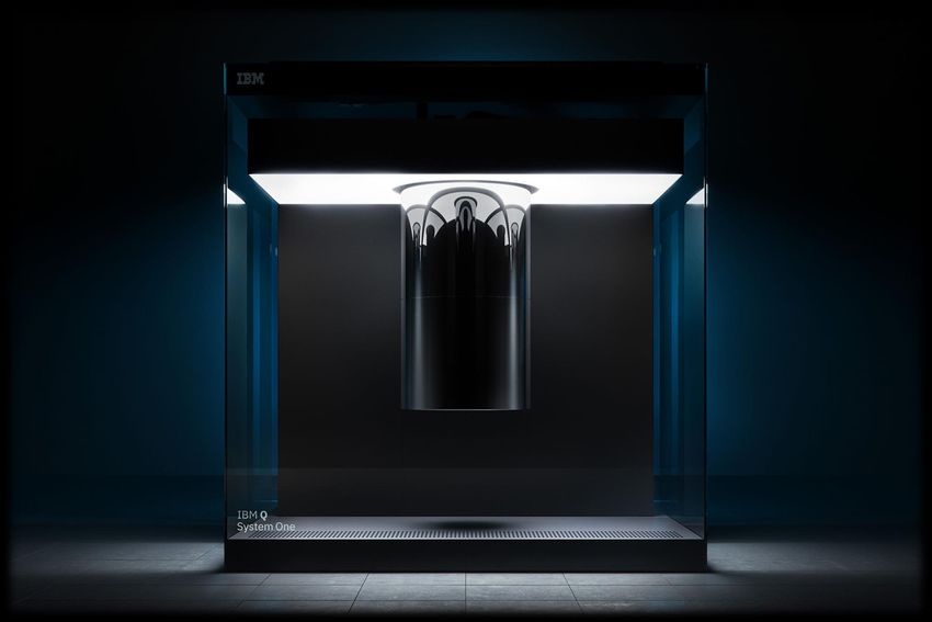

10
 Quantencomputer

Im Quantencomputer ersetzt man die kleinsten Informationseinheit Bit durch das Quantenbit (Qubit).

 e e
 Jedes
 klassische Ein Qubit hat zusäzlich
 Bit hat nur Superpositionszustände
 genau zwei (Kugeloberfläche)
 Zustände.

 g g

 Durch Verschränkung wird dieser Vorteil auf Operationen zwischen zwei Qubits übertragen.

 Für manche Aufgaben (Addieren, Multiplizieren) ist kein vorteilhafter Quantenalgorithmus
 bekannt  Macht nichts, dafür gibt es klassische Computer!

11
 Quantenbit & Bloch-Kugel

Classical bit  Deterministic, either in ground state “g” or in excited state “e”

Quantum bit (qubit)  Superposition of two computational basis states
 = g + e 
 | ⟩
 2
 , ∈ ℂ with ( ) + 2
 =1
  All states can be visualized on the
 surface of a sphere | ( )⟩
 ( )
Global phase unobservable
 Bloch sphere representation
 ( ) 
 ( ) ( )
 = cos e + ( ) sin g
 2 2

 Bloch angles 
  Amplitude  Energy, population | ⟩
 ( )  Phase  Coherence

12
 Pseudo spin and Pauli matrices

 Important states on the Bloch sphere
 Pseudo spin 
  | ⟩ equivalent to spin wavefunction | ⟩
 in external magnetic field
 − 
Unitary operations 
 Gates & evolution expressef via − 
 unitary operations ෡ 
 ෡
 | ⟩ expressed via the Hermitian
 + 
 Pauli spin matrices 1෠ , ො , ො , ො 
 + 
 1 0 0 1 
 1෠ ≡ ො ≡
 0 1 1 0
 
 0 − 1 0 | ⟩
 ො ≡ ො ≡
 0 0 −1
 ( ) ( )
 = cos e + ( ) sin g
 |g⟩ and |e⟩ are the eigenvectors of ො 2 2

13
Interpretation of the Pauli matrices

 Projection operators project the qubit state onto a certain basis state
  Example: g g selects all terms of with g
  Reason: g , e is orthonormal basis  g g = 1, g e = 0

 1 0 0 1 0 − 1 0
 1෠ ≡ ො ≡ ො ≡ ො ≡
 0 1 1 0 0 0 −1

 The Pauli matrices can expressed in terms of projection operators
 e
 ො+ = e g  Puts an excitation into the qubit g
 e
 ො− = g e  Removes an excitation from the qubit
 g
 ො = ො− + ො+ e
  Induce transitions between |g⟩ and |e⟩ g
 ො = ො− − ො+
 e
 ො = |e⟩⟨e| − g g  ⟨ ො ⟩ gives the qubit population ??
 g

 1෠ = |g⟩⟨g| + e e  Reflects normalization

14
 Single qubit gates

Examples for 1-qubit gates

Graphical representation example

 NOT

15
 Hadamard gate

 ෡ is of particular importance in many quantum algorithms
Hadamard gate 
  Applied to one of the basis states |g⟩ or |e⟩, it results in a superposition state of
 the basis states

 1 1 1 1
 ෡≡
 = ො + ො 
 2 1 −1 2
 | ⟩

 − 
 1
 ෡=
  e e − g g + e g + g e
 2 

 1
 ෡g =
 ( e − |g⟩)
 2 
 1 + 
 ෡e =
 (|e⟩ + |g⟩)
 2 

 | ⟩

Energy and phase relaxation 16

 (decoherence)
In practice, ideal unitary evolution is lost after some time due to
uncontrolled interaction with environment
 Loss os quantum coherence („decoherence“)
 ( ) ( )
 = cos e + ( ) sin g
 2 2
  Amplitude  Energy, population
 ( )  Phase  Coherence

 Population  Energy relaxation time 1 or r
  B ≪ ℏ ge  decay from |e⟩ to |g⟩
  Nonadiabatic (irreversible) processes
  Induced by high-frequency fluctuations ( ≈ ge )

 Phase  Pure dephasing time 
  Adiabatic (reversible) processes
  Induced by low-frequency fluctuations ( → 0)
  Often encountered: 1/f-noise
  Measurements always contain 1 -effects
 2−1 = 2 1 −1 + T −1
Nomenclature not always consistent in literature! Often „decoherence“ comprises both effects

17
 From single to multi-qubit systems
Singe qubit state  = 1 g + 2 |e⟩

Two qubit state  2 qubits A and B
  = 1 gg + 2 eg + 3 ge + 4 |ee⟩
  gg , eg , ge , |ee⟩ is orthonormal two-qubit basis
  gg shorthand for tensor product g A ⊗ g B

Two qubit operators  Tensor product of single qubit operators
 Example: ො A ⊗ ො B
  Matrix notation: Tensor product is blockwise product

Controlled NOT gate (CNOT)

18
 The Bell states

 The Bell states are of particular importance in many QIP protocols
 Created via a Hadamard and a CNOT gate

 ෡
 
 1
 00 00 ≡ 00 + 11
 2
 1
 01 01 ≡ 01 + 10
 2 ෡≡
 1 1 1
 
 1 2 1 −1
 10 10 ≡ 00 − 11
 2
 1
 11 11 ≡ 01 − 10
 2

 Nomenklatur: 0 ↔ g , 0 ↔ e

19
 Quantum vs. classical computing

Classical bits can be copied easily: C  CC

Quantum bits (quantum states) cannot be copied

 ෡ producing copies
 Proof: Assume that there is a unitary transformation 
 of | ⟩ and 
 ෡ 0 = and 
 ෡ 0 = | ⟩
 However, the quantum copying machine fails in copying state
 1
 0 = ( + | ⟩)
 2
 1
 ෡ 0 =
 ( + | ⟩) ≠ | ⟩
 2

 Rescues the consistency between quantum mechanics and special relativity
 No superluminal communication!

20
 Quantum teleportation
  No-cloning theorem forbids copying state = ↑ + ↓
  However, vanishing at one place and reappearing at another is allowed

 Teleporting a quantum state (qubit) requires that Alice and Bob share an entangled
 1
 state AB = ↑↓ + ↓↑ (“EPR pair”)
 2

 Teleportation protocol Alice
 1. Alice entangles her spin ↑ with the
 unknown state 
 2. Alice measures what state her two spins are and
 tells Bob, which of the four possible results
 she has found
  Classical communication
 3. Bob carries out the appropriate rotation of his spin ↑ by Bob
 4. As a result, Bob ends up with his spin in the state = ↑ + ↓

21
 Primfaktorenzerlegung

 Öffentlicher & privater Schlüssel basieren auf (demselben) Produkt zweier Primzahlen
 Verschlüsselung mit öffentlichem Schlüssel & Entschlüsselung mit privatem Schlüssel
 Kenntnis der Primzahlen erlaubt Rekonstruktion der Nachricht aus öffentlichem Schlüssel

  Schnellere Faktorisierungsalgorithmen strategisches Interesse vieler Staaten

 Problemgröße  Stellenzahl = log der zu faktorisierenden Zahl 
Klassischer Computer (Zahlkörpersieb) Quantencomputer (Shor-Algortihmus)
 2
 1Τ3 log 3  Laufzeit ∝ 3
  Laufzeit ∝ 
 1 1  Polynomiell
 32 3 64 3
  = , 9 ≃2
 9
 (implementierungsbhängig)
  Subexponentiell
 Peter W. Shor
  Leider trotzdem superpolynomiell

22
 Primfaktorenzerlegung
 Problemgröße  Stellenzahl = log der zu faktorisierenden Zahl 

 1 1
Lehmer-Powers continued fraction or via
 Laufzeit exp 2 log 
 2 2
the Kraitchik polynomial

 2
Pollard’s method 1Τ3 log 3
  Laufzeit 
 1 1
 32 3 64 3
  = , 9 ≃2
 9

Shor’s algorithm Laufzeit 3 Gatteroprationen

  Taktfrequenz, Zeit pro Gatteroperation, Parallelisierung etc.
  Für große Probleme ist der Quantenalgorithmus immer viel schneller
  Aber: Wenn die Quantenhardware zu schlecht ist, hilft der Quantenvorteil in
 der Praxis nicht

23
 Weitere Quantenalgorithmen

Anwendung Quantenalgorithmus Quantenvorteil
Datenbanksuche Grover-Algorithmus ∝ anstatt ∝ 
Lin. Differentialgleichungen HHL-Algorithmus ∝ log anstatt ∝ 
Optimierungsprobleme Quantenannealing Polynomiell statt
• Handlungsreisender exponentiell
• Warenströme
• Verkehrsprobleme
• Risikoanalyse
Quantenchemie Quantensimulation mit statt 2 Prozessor- oder
• Katalysatoren leicht kontrollierbarem Speicherelemente
• Medizin Quantensystem
• Materialforschung

Universal quantum processor: 24

 Required elements

 Qubit 2 qubit gates (e.g., C-NOT)
 (two-level
 (controlled interactions)
 quantum system)

 e e e
 g e
 g g g

 read out

 U1 U1 U1 Useful: Quantum memories

Single qubit gate

25
 Hardware-Plattformen
Quantenhardware – Herausforderungen
• Viel empfindlicher gegen kleinste Störungen als klassische Hardware
• Komplizierte und weniger reproduzierbare Herstellung
• Großer Fehlerkorrekturoverhead (Qubits × 1000) beeinträchtigt Skalierbarkeit
• Initialisierung, Kontrolle, und Auslese aufwendig
 Riesige Diskrepanz zwischen verfügbaren Quantensystemen (5-70 nicht fehlerkorrigierte
 Qubits) und algorithmischen Erfordernissen (Millionen fehlerkorrigierte Qubits)

Zahlreiche Realisierungsmöglichkeiten
• Supraleitende Quantenschaltkreise
• Ionenfallensysteme
• Quantencomputer auf Diamantbasis
• Quantencomputer auf Basis von Halbleiter-Quantenpunkten
• Marjorana-Systeme
• ...

26

Quantencomputing mit
 supraleitenden
 Schaltkreisen

27
 Supraleitende Quantenschaltkreise
 Supraleitung
 
 Aluminuim
 Τℎ ≃ 50 GHz
 ≪ B 

 e
 q
 F g

 Quantenressourcen:
 Mikrowellen Superpositon & Verschränkung
 ≃ −

 5 − 10 GHz −
 − + 

  Quantencomputing, Quantensimulation,
 Quantensensing
 Millikelvin-
 temperaturen
 1GHz ⇔ 50 mK

28
 Fundamentale Quantenschaltkreise
 -Resonator  Box für Quantenmikrowellen
 |2⟩
 |1⟩ r
 2 0 r
 =
 1
 2 
L r =
 
 C 2 ෡ ෠ = ℏ
 ,
 = ℏ r > 
 2 „Quantum 2.0“

 10 mm

Applications of quantum harmonic 29

 oscillators

Quantum HO is linear  Not a qubit  Not directly useful for quantum computation!

 Nevertehless indirect use:
 Quantum
 simulation of Mediate coupling
 manybody between qubits
 Hamiltonians  Quantum bus

 Qubit readout
 L C Typically long
 („dispersive coherence times
 readout“)  Quantum memory

 Ancilla qubit/nonlinearity Identify
  Explore quantum decoherence sources in
 physics (Fock states, superconducting
 squeezing etc.) quantum circuits

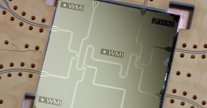
30
 Fundamentale Quantenschaltkreise

 SIS Josephsonkontakt
L J

 Josephsonindutivität 
 Nichlinear, kann negativ sein, mit Magnetfeldern steuerbar

 |e⟩
 J C q
 |g⟩

 Supraleitendes Künstliches Zweiniveauatom
 Transmonqubit

31
 The transmon qubit
J. Koch et al., Phys. Rev. A 76, 042319 (2007).
 Embed into a resonator for
  Readout
  Filtering
  Control

 Currently most successful qubit
 with respect to coherence times

 Coherence mostly limited by
 spurious TLS (defects) in substrate
 and metal-substrate interface

  T1 , T2 ≃ 50 − 150 μs

32
 Dispersive readout
 Use resonator as readout device
  Off resonance  Qubit resonator coulping induces qubit-state-dependend shift of the
 resonance frequency 2 ℏ g2 int
 ෡JC
 =ℏ ෝ ෝ
 †ෝ
 + ෝ 
 ≡ q − r
 2 

 e g
 Transm. phase
 Transmission
 magnitude

 2 2
 r + r − Frequency
 
 2 2 2 Frequency
 q + r + r −
 
 Two-tone spectroscopy
 2
  Send probe tone rf = r + 
  Sweep spectroscopy tone s
  Qubit is in e  Transmission magnitude will drop drastically from blue to green curve
  Mixed state  Reduced shift, but still ok
  Transmission phase can also be used!

33
 Qubit control
Qubit Hamiltonian equivalent to that of a spin in a static magnetic field
 Use NMR techniques to control qubit on Bloch shere
 Rotating field in euqstorial plane of the Bloch shere  Population oscillations
 In practice, oscillating (microwave) fields are used
 
 | ⟩
 ෩
 | ( )⟩
 ( )
 | ⟩
 
 | ( )⟩
 
 | ⟩ ෩ = | ⟩
 
 Phase control Population control
  Free (Larmor) precession  Equatorial microwave drive field

34
 Rabi (population) oscillations
Drive qubit with microwave field On resonance = q
  Rotating frame cancels Larmor precession
 Δ 2 + d2 ෩ has no -evolution
  State vector 
 d2
 e = sin2  ෩ = cos d g + sin d e
 Δ 2 + d2 2 2 2
  Rotation about -axis

 Finite detuning Δ > 0 
  Additional precession at 
 Population oscillates faster ෩
 | ( )⟩
  Reduced oscillation amplitude

 4

 3
 
 2 Τ d

 2

 1

 0
 
 −5 0 5 ෩ = | ⟩
 
 d

Important drive pulses 35

 on the Bloch sphere
 2 / 

 2ℏ d

 Δ 
 
 − + 
 
 | ⟩
 -pulse ( d Δ = ) /2-pulse ( d Δ = /2)
g ↔ |e⟩ flips, refocus phase evolution Rotates into equatorial plane and back

Energy relaxation 36

 and driven Rabi oscillations

A. Wallraff et al., Phys. Rev. Lett 95, 060501 (2005)

Energy relaxation 37

 and driven Rabi oscillations

A. Wallraff et al., Phys. Rev. Lett 95, 060501 (2005)

∗ 38
 Ramsey fringes ( )

A. Wallraff et al., Phys. Rev. Lett 95, 060501 (2005)

39

 Nationale und
 Internationale
Forschungsaktivitäten

Quantenwissenschaften & -technologie
Extrem kompetitives Forschungsgebiet an internationalen Spitzenplätzen!

EU Quantenflaggschiff

 https://qt.eu/

WMI koordiniert Projekt “Quantum microwave communication
and sensing” & baut weltweit erstes Q-LAN im Mikrowellenbereich

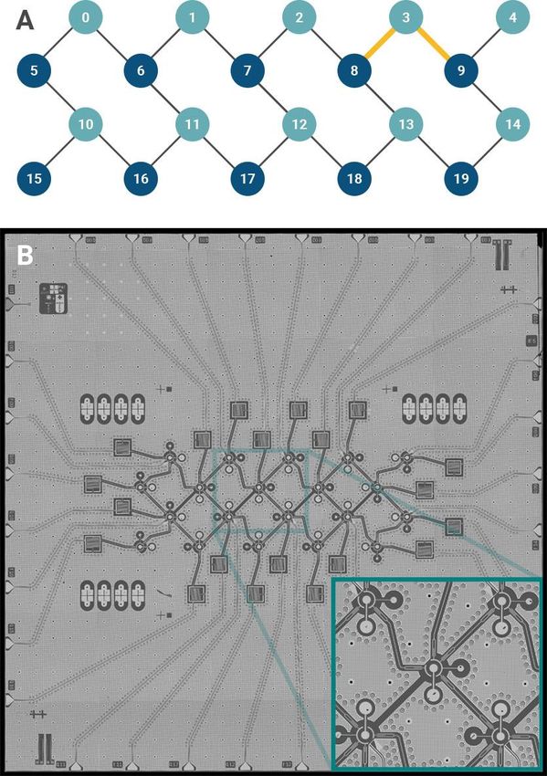
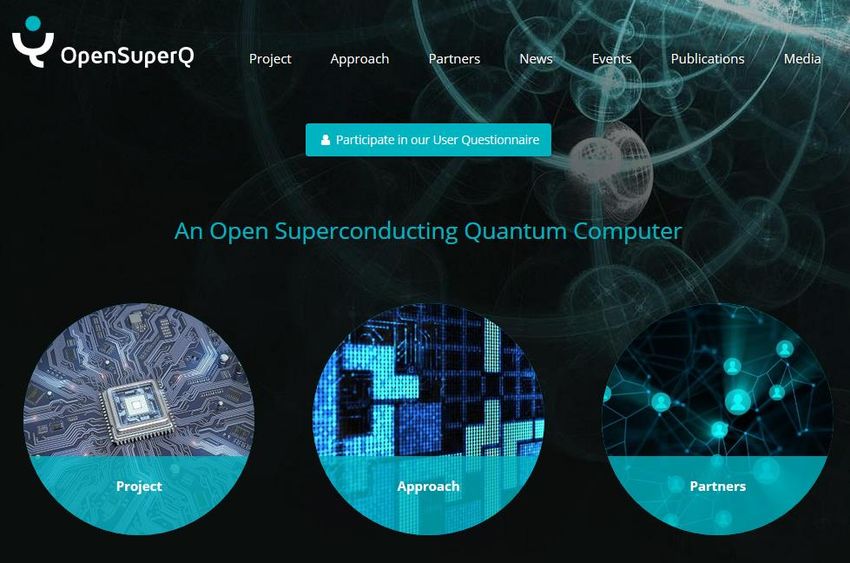
Supraleitendes Quantencomputing im 42

 EU-Flaggschiff

Supraleitende Schalkreise in München

 Sonderforschungsbreich 631 (2003-15)
 Festkörperbasierte Quanteninformationsverarbeitung

 Exzellenzcluster Nanosystems Initiative Munich (2006-18)
 Forschungbereich 1: Quantum Nanophysics

 Graduiertenschulen:
 Exploring Quantum Matter (2014-22)
 Quantum Science & Technology (2016-21)

 Münchener Quantenzentrum (seit 2014)
 TUM, LMU, MPG, BAdW

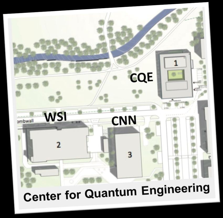
Quantenengineering@ München

Forschungsbau: ca. 40 Mio. € Exzellenzcluster: ca. 9 Mio. € / Jahr
Fertigstellung: ca. 2022 Förderzeitraum: 2019 - 2025

MCQST – Zielsetzungen
 Skalierbare Quantencomputer
 Schlüsselkomponenten, neue Architekturen, Software, …

 Quantensimulatoren
 >10 000 Qubits, programmierbar, verbesserte Kontrolle, …

 Quantenkommunikation
 sicher, skalierbar, Basis für Quanteninternet, …

 Hybride Quantensysteme
 Schnittstellen zwischen Technologieplattformen, topologische Systeme, ….

 Kontrolltechnologie für Quantensysteme
 optimale Kontrolle, Vielteilchensysteme, …

 Quellen für Quantenlicht & Quantensensoren
 für Anwendungen in Metrologie, Quantennetzwerken, Biologie, Medizin, …

 Quantenmaterialien
 maßgeschneiderte Materialein, neuartige Quantenbits, …

Exkurs: Quantenkommunikation und 46

 –sensorik mit Mikrowellen

 C

47

Industrielle Aktivitäten
 zu supraleitenden
 Quantenschaltkreisen

IBM Quantum Experience

 Gatterpräzision > 99.6%

 https://quantumexperience.ng.bluemix.net/qx/devices

IBM Q System One
 20 qubit machine

CES Las Vegas, January 2019

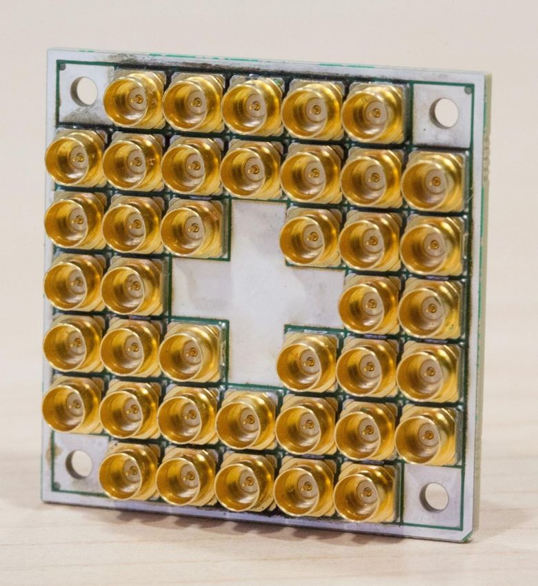
Intel Delivers 17-Qubit Superconducting Chip

 Oct. 2017:

 chip with advanced
 packaging delivered to
 QuTech

 Intel’s 17-qubit superconducting
 test chip for quantum computing
 has unique features for improved
 connectivity and better electrical
 and thermo-mechanical
 performance.

Google has lifted the lid on its new quantum processor,
 Bristlecone. The project could play a key role in making
 quantum computers "functionally useful."

72 qubit processor

Rigetti Quantum Comnputing

 Januar 2019:
19-Qubit-Chip Rigetti Cloud
 Service

Viele Quantum Software Startups

Zukunftsvisionen

Für die Pessimisten...

 Langzeitvorhersagen...
“I think there is a world market for maybe five computers”
Thomas J. Watson, chairman of IBM, 1943

“Whereas a calculator on the Eniac is equipped with 18000 vacuum tubes and weighs 30
tons,
computers in the future may have only 1000 tubes and weigh only 1½ tons”
Popular Mechanics, March 1949

“There is no reason anyone would want a computer in their home”
Ken Olson, president, chairman and founder of DEC, 1977

 ... sind meistens falsch !!!

56

Epilog: Supraleitende
Quantenschaltkreise
Quantenmikrowellen

Exkurs: Supraleitende 57

 Quantenschaltkreise am WMI
Grundlagen für Quantencomputing Quantenkommunikation und -sensorik
 und -simulation mit Mikrowellen

 Licht-Materie-Wechselwirkung Quantenmikrowellenphotonik

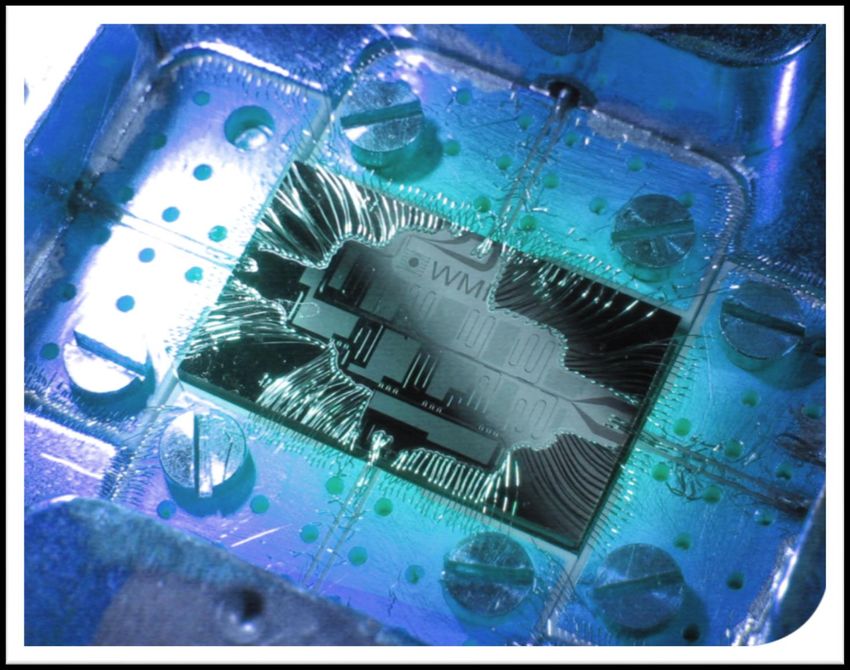
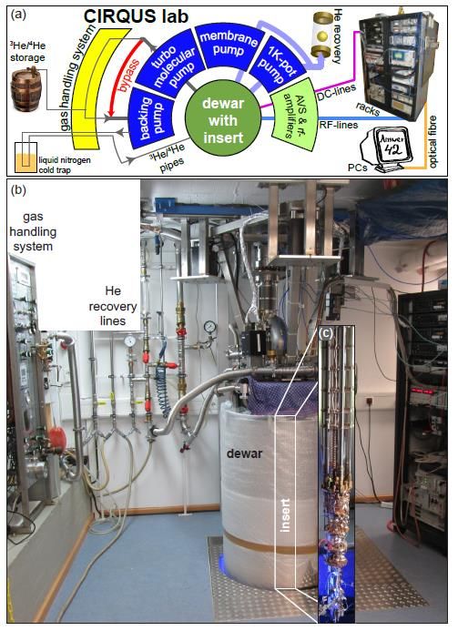
58
Typische Setups

59
Typische Setups