Potential of Greenland cockles (Serripes groenlandicus) as high resolution Arctic climate archive

Potential of Greenland cockles
 (Serripes groenlandicus) as high
 resolution Arctic climate archive
 Potential der Grönlandherzmuschel (Serripes groenlandicus)
 als hochauflösendes Klimaarchiv der Arktis

 Masterarbeit im Studiengang Meeresbiologie zur
 Erlangung  des  Titels  „Master  of  Science“
 Angefertigt von Verena Merk in der Sektion Bentho-Pelagische-Prozesse am Alfred-
 Wegener-Institut Helmholtz-Zentrum für Polar- und Meeresforschung, Bremerhaven

 Matrikelnummer: 212209132
 Wohnort: Verdener Str. 29a, 27570 Bremerhaven
 Abgabe: 18. März 2015

 Erstgutachter: Prof. Dr. Gerhard Graf, Universität Rostock
Zweitgutachter: Dr. Jürgen Laudien, Alfred-Wegener-Institut Helmholtz-Zentrum für Polar-
 und Meeresforschung, Bremerhaven

 Bremerhaven März 2015

Titelbild: G. Veit-Köhler

Zusammenfassung
 Um die klimatische Zukunft der Erde vorauszusagen ist das Wissen um ihre Vergangenheit
unabdingbar. Klimamodelle, die mögliche Entwicklungen des zukünftigen Klimawandels
modellieren, basieren auf Daten früherer Umweltbedingungen. Die Verlässlichkeit dieser
Klimamodelle ist abhängig von der Qualität und Quantität dieser Daten. Da Messungen nur
begrenzt zur Verfügung stehen werden Klimaarchive herangezogen um die
Umweltbedingungen der Vergangenheit zur rekonstruieren. Archive zeichnen, für den
Zeitraum ihrer Entstehung, indirekte Informationen über ihre Umgebung auf. Ist die Beziehung
zwischen einem, in einem Archiv aufgezeichneten, Stellvertreterparameter und einem
Umweltparameter bekannt kann dies als so genannter Proxy verwendet werden. Bivalvien sind
möglich Archive, die durch die Veränderungen von Wachstumsraten und Schalencarbonat
Zusammensetzungen Rückschlüsse auf das umgebende Meerwasser zulassen. Ein möglicher
Proxy ist dabei das Verhältnis von 18O zu 16O (δ18O) Isotopen im Schalencarbonat. Für die
meisten Bivalvien ist das Gleichgewicht zwischen δ18O Werten des Schalencarbonats und des
umgebenden  Meerwassers  abhängig  von  Temperatur  und  Salinität.  Um  die  δ18O Werte des
Schalencarbonates einer Muschelart als Proxy nutzen zu können muss die Möglichkeit
ausgeschlossen werden, das metabolische Prozess das Gleichgewicht der δ18O Werte
beeinflusst. Dafür müssten δ18O Werte des Schalencarbonats einer Muschelart mit
gemessenen Meerwasserparametern kalibriert werden. Die zirkumpolar
Grönlandherzmuschel Serripes groenlandicus (Bruguiere, 1789) war bereits in der
Vergangenheit Gegenstand stabiler Isotopen Analysen. Jedoch wurde bisher keine
Kalibrierung durchgeführt. Die vorliegende Arbeit untersuchte ob die im Schalencarbonat von
S. groenlandicus gemessenen δ18O Werte von metabolischen Prozessen beeinflusst werden.
Dafür wurden 37 Individuen einer Population in Kongsfjorden (Spitzbergen) entnommen. Die
Schalen von drei Individuen wurden zur Analyse stabiler Isotopen herangezogen. Die
gemessenen δ18O Werte der Schale wurden anschließend mit berechneten δ18O Werten
verglichen. Die berechneten δ18O Werte beruhten auf Temperatur- und Salinitätsmessungen
in der direkten Umgebung der S. groenlandicus Population. Um zu zeigen, dass die, für die
Analyse der stabilen Isotope ausgewählten Individuen repräsentativ für die Population sind,
wurden ihre Wachstumsraten mit den der ebenfalls gesammelten Individuen verglichen.
Zudem wurde festgehalten zu welchem Zeitpunkt die Muscheln dunklere Inkremente
(Wachstumslinien) in ihre Schale einbauen. Mit Hilfe eines Konfokalen Raman Mikroskops und
eines Rasterelektronenmikroskops wurde die Struktur des Schalencarbonates überprüft. Die
Ergebnisse zeigen, dass die Wachstumsraten aller gesammelten Individuen vergleichbar
waren. Die Überprüfung der Wachstumslinien ergab, dass diese im Spätsommer bis Herbst
gebildet wurden. Es konnte außerdem gezeigt werden, dass die Schalenstruktur von S.
groenlandicus aragonitisch ist. Allerdings zeigte sich an manchen Stellen auch eine erhöhte
Porosität. Die Analyse stabiler Sauerstoff Isotope des Schalencarbonates ergab, dass eine
große   Ähnlichkeit   zwischen   gemessenen   und   berechneten   δ18O Werten gab. Berechnete
Minimalwerte wurden dabei nicht in der Schale aufgezeichnet. Die lässt vermuten, dass das
Wachstum von S. groenlandicus entweder von höheren Temperaturen oder geringer Salinität
gehemmt wurde. Aus diesen Ergebnissen wurde geschlossen, dass das Gleichgewicht
zwischen δ18O Werten des Meerwassers und des Schalencarbonates nicht durch
metabolischen Prozesse beeinflusst wird. Zusätzlich war es möglich die Schalen durch
manuelles fräßen der Proben hochauflösend zu beproben (65µm).
 I

Abstract
 In order to predict the climatic future of the earth, knowledge about the past is
indispensable. Climate models which predict possible developments of future climate change
are based on data of past environmental conditions. The precision of these climate models
depends on quality and quantity of those data. Since recent measurements are limited, climate
archives are used to reconstruct past conditions. Archives indirectly provide information about
the surrounding environmental conditions at the time of their formation. Once the relationship
between a representative parameter recorded by an archive and an environmental parameter
is known this could function as a so called proxy. Bivalves are possible archives recording
ambient seawater parameter incrementally as a variation of growth rates or shell calcium
carbonate (CaCO3) composition. A potential temperature proxy is the ratio of 18O/16O  (δ18O)
recoded in the shell carbonate of some Bivalves. The equilibrium between recoded and
measured δ18O of the seawater is determined by temperature and salinity. In order to use this
recording of δ18O in shell carbonate it is necessary calibrating δ18O of the seawater with
measurements of surrounding seawater parameters to exclude the possibility of metabolic
influences on this equilibrium. The Greenland cockle Serripes groenlandicus (Bruguiere,
1789), a bivalve occurring circumpolar has already been a subject to stable oxygen and carbon
isotopes analyses. However, a calibration have not been provided yet. This study investigated
whether the equilibrium between δ18O measured subsequently in shell carbonate of
S. groenlandicus and the ambient seawater is influenced by metabolic processes. Therefor the
shells of 37 specimens, were collected from a population located in Kongsfjorden
(Spitsbergen). Three of them were used to subsequently measure δ18O values of shell
carbonate  and  compared  to  predicted  δ18O  shell  values.  The  predicted  δ18O values of the shell
were calculated from temperature and salinity measurements of the ambient seawater. Growth
line deposition and growth rate were examined in specimens of the same population in order
to prove that the three individuals chosen for stable isotope analysis are representative for this
population regarding their growth pattern. Additionally the structure of shell carbonate was
analyzed using a Confocal Raman microscope and a scatter electron microscope. Results
prove, that the individuals chosen for stable isotopes analyses were representative individuals
of the population regarding their growth rate. The evaluation of growth line deposition
examined in all collected shells showed a deposition in late summer up to fall. It was also
proven that the crystalline structure of the shell carbonate was aragonite. However, embedding
shells in Araldite showed the occurrence of a porous structures in the outer shell layer. Stable
oxygen isotope analysis and comparison with ambient conditions during shell formation prove
a strong similarity between predicted and measured δ18O values of the shell where an
alignment was possible. However, the minimum of predicted δ18O values was not recoded in
the shell carbonate, indicating that the growth of S. groenlandicus is limited by either high
temperature or low salinity. The  total  range  of  δ18Oshell values  was  3.53‰.  From these findings
it was concluded, that the equilibrium between shell stable oxygen isotope ratios is not
influence by metabolic processes. It was furthermore noted that a high resolution sampling (68
µm) of shell carbonate of S. groenlandicus by manual milling possible.

 II

________________________________________________________________

Content

 Zusammenfassung.............................................................................................. I
 Abstract............................................................................................................... II
 Abbreviations and acronyms ............................................................................ V
 List of Tables ..................................................................................................... VI
 List of Figures ................................................................................................... VI
 1 Introduction ............................................................................................ 1
 2 Objectives .............................................................................................. 6
 3 Materials and methods .......................................................................... 7
 3.1 Study site ............................................................................................... 7
 3.2 Shell collection and environmental data ............................................. 9
 3.3 Shell preparation ................................................................................. 10
 3.4 Representativeness of individual growth .......................................... 11
 3.4.1 Growth line deposition ........................................................................... 11
 3.4.2 Growth rate ............................................................................................ 13
 3.5 Crytalline structure of the shell carbonate ........................................ 14
 3.5.1 Confocal Raman microscopy ................................................................. 14
 3.5.2 Electron microscopy .............................................................................. 16
 3.6 Stable oxygen and carbon isotopes .................................................. 17
 3.6.1 Sampling of biogenic calcium carbonate of shells ................................. 17
 3.6.2 Measurment of stable oxygen and carbon isotopes .............................. 19
 3.6.3 Alignment of measured and calculated δ18O values .............................. 19
 4 Results.................................................................................................. 21
 4.1 Representativeness of individual growth .......................................... 21
 4.1.1 Growth line deposition ........................................................................... 21
 4.1.2 Growth rate ............................................................................................ 22
 4.2 Crystalline structure of the shell carbonate ...................................... 24
 4.2.1 Confocal Raman microscopy ................................................................. 24
 4.2.2 Electron microscopy .............................................................................. 27
 4.3 High resolution sampling of calcium carbonate ............................... 29
 4.4 Oxygen and carbon stable isotopes .................................................. 29

 III

________________________________________________________________
5 Discussion ........................................................................................... 35
5.1 Representativeness of individual growth .......................................... 35
5.2 Crystalline structure of the shell carbonate ...................................... 35
5.3 High resolution sampling of calcium carbonate ............................... 36
5.4 Oxygen and carbon stable isotopes .................................................. 37
6 Conclusion and outlook ...................................................................... 39
7 References ........................................................................................... 40
8 Declaration ........................................................................................... 44
9 Acknowledgment ................................................................................. 45

 IV

________________________________________________________________

Abbreviations and acronyms
δ Delta
δ13C Stable carbon isotope ratio of 13C to 12C
δ18O Stable oxygen isotope ratio of 18O and 16O
δ18Opredicted Predicted stable oxygen isotope ratio of the shell carbonate
δ18Os Stable oxygen isotope ratio influenced by salinity
δ18O shell Stable oxygen isotope ratio of the shell carbonate
12C Stable isotope of carbon with 12 neutrons
13C Stable isotope of carbon with 13 neutrons
18O Stable isotope of oxygen with 18 neutrons
16O Stable isotope of oxygen with 16 neutrons
a Year
ArW Arctic Water
AWI Alfred-Wegener-Institut
 Helmholtz-Zentrum für Polar- und Meeresforschung
C Carbon
CaCO3 Calcium carbonate
CO2 Carbon dioxide
CRM Confocal Raman microscopy
DOG Direction of growth
e.g. exempli  gratia,  Latin  for  “for  example”
et al. et alii, Latin for “and  others”
IPCC Intergovernmental Panel on Climate Change
IRMS Isotope ratio mass spectrometer
k Growth constant
NAO North Atlantic Oscillation
O Oxygen
pH Negative logarithm of the hydrogen ion concentration
R2 Error square
S. groenlandicus Serripes groenlandicus
SEM scattering electron microscope
SH∞ Asymptotic maximum shell height
SHt Shell height at time t
Ssea Salinity of the seawater
t Time in years
t0 Time when shell height was theoretically zero
Tsea Temperature of the seawater
VPDB Vienna Peedee Belemnite
WSC West Spitsbergen Current

 V

________________________________________________________________

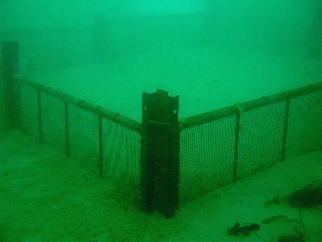
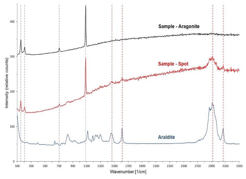
List of Tables
Table 1. Verification of the calcein lines, differentiated between umbo and shell. .................21
Table 2. S. groenlandicus: List of carbonate samples taken from three shells.
.............................................................................................................................................29

List of Figures
Figure 1: Overview of the shell morphology of the Greenland cockle S. groenlandicus ......... 5
Figure 2: Map of Spitsbergen and the Kongsfjorden-Krossfjorden system ............................. 8
Figure 3: Enclosure (3 x 3 m) where the population of Greenland cockles was held. ............10
Figure 4: Incubation of Greenland cockles in 100 mg l-1 calcein solution. ............................11
Figure 5: Examples for calcein lines under reflected and fluorescent lights ..........................12
Figure 6: S. groenlandicus: Measurement of the width of two increments using AnalySIS 5.0
 software. ............................................................................................................13
Figure 7: Rayleigh and Raman scattering .............................................................................15
Figure 8: Sampling of calcium carbonate for stable isotopes analysis ..................................18
Figure 9: Number of increments per year and ontogenetic shell age. ...................................23
Figure 10: Shell height-at-age data for the shell taken for the S. groenlandicus sub-population,
 including von Bertalanffy growth function ...........................................................23
Figure 11: Confocal Raman microscopy map and spectrum of shell cross sections of
 S. groenlandicus. ...............................................................................................24
Figure 12: Different images of the shell structure of S. groenlandicus ..................................26
Figure  13:  CRM  spectra  of  a  region  with  ‘spots’....................................................................27
Figure 14: Scanning electron microscope images showing cross sectioned shell of S.
 groenlandicus .....................................................................................................28
Figure  15:  δ18Oshell values for all three individuals displayed with equal spacing ...................31
Figure 16: Seawater temperature, salinity and δ18Opredicted at the study site ..........................32
Figure  17:  Alignment  of  δ18Oshell  and  δ18Opredicted values......................................................33
Figure  18:  δ13C values of shell carbonate taken from S. groenlandicus shells ......................34

 VI

Introduction
__________________________________________________________________________

1 Introduction
 Throughout the 4.5 billion years of its existence the earth experienced a broad variety of
changes, including changes in the composition of the atmosphere (Catling and Claire 2005),
the origin and evolution of life (Baross and Hoffman 1985) and the movement of continents
related to plate tectonics (Wegener 1912). Furthermore, extensive variations in climatic
conditions let to transitions between glacial and interglacial periods (e.g. Rogers 1993). The
understanding of how and why global and local climatic conditions changed in the past
provides the possibility to understand and identify the major forces involved in this process
(IPCC 2013). Additionally, by looking at the past we can predict how the biosphere and coupled
mechanisms may react to a specific change in the climate system. The polar regions in
particular reacts very sensitive to such variations due to polar amplification. Meaning the
melting of snow and ice exposes ocean and land surfaces that absorb solar radiation much
more effective. Thus they will heat up causing further melt of ice and snow which again would
expose more ocean and land surfaces. The Arctic in particular is more sensitive than the
Antarctic since its temperatures are near to the melting point (Miller et al. 2010; Serreze and
Francis 2006)
 The knowledge about environmental conditions of the past (e.g. climate) is based on data
such as ocean and land temperature, salinity and pH of seawater. Since recent measurements
are limited in times they are combined with reconstructed data to verify climate models. Those
climate models can for instance be used to predict the anthropogenic induced climate change
the earth is about to face in the near future (IPCC 2013).
 Climate models are numerical models, which intend to predict the future development of
important environmental parameters (e.g. global temperatures) based on various assumptions
such as the future anthropogenic emissions of carbon dioxide (CO2). Their precision relays on
the comparison to modeled past conditions with reconstructed (proxy data) or measured
parameters. Furthermore, the accuracy depends on quality and the temporal resolution of the
reconstructed and measured data. The better the amount, continuity, resolution and certainty
of the data available, the better the reliability of the climate model (Fischer and Wefer 1999;
IPCC 2013).
 In order to reconstruct past environmental and climatic conditions many different archives
and proxy data are used. Archives indirectly provide information about the surrounding
environmental conditions. At the time of growth or deposition different archives can indirectly
record distinct environmental parameters, such as temperature or salinity (Versteegh et al.
2012). Once a correlation between such a representative parameter (proxy) and an
environmental condition is identified and understood, this proxy can be used to reconstruct

 1

Introduction
__________________________________________________________________________
paleo-climatic or -environmental information. Since different archives provide data in spatially
and temporally limited ranges, data sets need to be complementary. Archives can be biogenic
such as bivalves, trees, corals, coralline algae, fish otoliths and or non-biogenic such as the
composition of ice or sediments cores (e.g. Fischer and Wefer 1999; IPCC 2013).
Environmental information archived through biogenic proxies can be retrieved from the
variability of growth patterns (e.g. annual growth rates of bivalves) or the biogeochemical
composition of bio-minerals (e.g. stable isotope ratios or trace and minor elemental ratios from
shell carbonate) (Fischer and Wefer 1999).
 All physical and chemical studies of incrementally and chronological features in biological
hard tissue of marine and freshwater organisms can be referred to as sclerochronology (Jones
1983). Organisms known to grow discrete are bivalves (e.g. Richardson 2001). Since their
shell growth is asymptotic they record environmental conditions over their whole lifespan
(Richardson 2001). Bivalves grow by secreting calcium carbonate (CaCO3) and thus extending
their shell towards the ventral margin (Richardson 2001). Most shells follow a pattern of
alternating lighter and darker bands, which may be prominent in cross sections, as well as on
the outer shell surface (Richardson 2001). In many bivalve species the thinner, but darker
bands or growth lines are known to form annually (e.g. Ambrose et al.   2006;;   Bušelić   et al.
2014). Due to unfavorable conditions, such as low water temperatures or a lack of food, the
shell secreting mantle edges are retracted from the margins (Richardson 2001). As a
consequence growth slows down or stops (Richardson 2001). Once it has been proven that
the darker growth lines are built annually they can be used for age determinations. If conditions
are more favorable shells grow at a higher rate (Richardson 2001). This results in wider and
lighter increments, which are built gradually over the growth period. The overall annual growth
of bivalves is determined by their biology, the ontogenetic age and environmental conditions
such as temperature and nutrient supply (Jones et al. 1989; Schöne 2013). In general, more
favorable conditions lead to wider annual increments. This concept was used extensively in
standardized growth models to correlate shell growth with environmental events (Ambrose et
al.  2006;;  Bušelić  et al. 2014; Schöne 2008). Once established, such a correlation can be used
as a proxy to reconstruct past environmental conditions for selected geographic regions
(Marchitto et al. 2000).
 Despite using morphological features it is also possible to receive information from the shell
material itself. The biogeochemical composition of the shell carbonate is determined by a
variety of physical and chemical properties of the ambient seawater. Thus, stable isotope
geochemistry is implemented frequently in paleontological studies (Wassenaar, Brand, and
Terasmae 1988). In order to use stable isotope ratios for the reconstruction of ambient

 2

Introduction
__________________________________________________________________________
conditions, the influences of different parameters such as seawater temperature, salinity or
metabolic processes of the organism need to be understood (Schöne 2008).
 Stable  carbon  isotope  ratios  (δ13C) potentially contain information about water properties
related to primary production. However, the biological influence on its incorporation into the
shell carbonate is not yet fully understood and therefore it is not possible to reliably interpret
them  (for  details  on  δ13C in bivalves see Gillikin et al. 2007; Romanek et al. 1992).
 In contrast, for the stable oxygen isotopic composition much is already known about the
mechanisms (e.g. Epstein and Mayeda 1953). As the ratio of 18O/16O (δ18O) is inversely linked
 18 16
to temperature (Epstein et al. 1961) changes in the ratio of O to O is theoretically mainly
caused by thermodynamic processes. The changes in the ration of 18O to 16O is referred to as
fractionation.
 In reality this fractionation is much more complex, especially in marine environments.
Evaporation  effects  δ18O since the lighter 16O is more likely to change into vapor phase (Epstein
 18
and Mayeda 1953). Conversely, O is more prominent in precipitation. An additional factor in
marine environment is the difference between seawater and freshwater. In general, changes
in salinity  affect  δ18O in similar ways but not equally pronounced (Epstein and Mayeda 1953).
The  δ18O values of freshwater are much lower and they also differ between sources. The  δ18O
values of for example melted snow are much more negative than the values of a river inflow
not fed by meltwater. Thus the negative influence of an inflow fed by meltwater on  the  δ18O of
seawater is higher, than the one cause by a river inflow not fed by meltwater, however, both
events will lower salinity likewise (Epstein and Mayeda 1953). This leads to ocean waters with
the   same   salinity,   but   different   δ18O (Epstein and Mayeda 1953). In order to work with the
relationship   between   salinity   and   δ18O it is necessary to determine it for each study area
(Maclachlan et al. 2007).
 The real paleontological value of variations in stable oxygen isotope compositions is based
on the knowledge of how they are incorporated into the biogenic carbonate. Without any
metabolic inference the incorporation into the shell carbonate is in equilibrium with the ambient
δ18O of the seawater. This relationship however depends on the polymorphs of calcium
carbonate (for bivalves mostly calcite or aragonite) (Epstein and Mayeda 1953; Grossman and
Ku 1986). Once proofed for a particular species, that there are no metabolic processes
influencing the δ18O it can be used as a temperature proxy  wherever  δ18O of the seawater or
its correlation with salinity is known (Schöne and Fiebig 2009).
 In the past this approach has been used for different calcifying organisms such as bivalves
or calcifying foraminifera (Versteegh et al. 2012; Zachos et al. 1996). However, some bivalves
have, despite a long lifetime and global distribution one crucial advantage: The incremental
shell accretion allows for an examination of the variation in carbonate composition on an intra-

 3

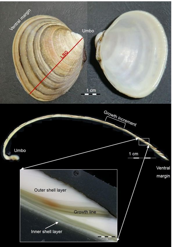
Introduction
__________________________________________________________________________
annual scale (Richardson 2001). This enables the possibility to resolve seasonal patterns
within the shell (Hallmann et al. 2008, 2009; Khim et al. 2001; Versteegh et al. 2012).
 Khim (2002) and Khim et al. (2003) used shells of the Greenland cockle Serripes
groenlandicus (Bruguiere, 1789) to reconstruct seawater temperatures and salinity of
seawater. He concluded that there are no metabolic changes to the stable oxygen isotope
incorporation by the animal. However, for the potential Arctic bio-archive S. groenlandicus this
proof and calibration have not yet been provided directly.
 S. groenlandicus is an infaunal suspension feeder. Populations of this cockle occur
circumpolar in the Arctic up to the boreal regions and can be found from the subtidal zone
down to 100 m water depth (Khim 2001; Kilada et al. 2007). In recent years this cockle species
became a valuable by-catch in the fishery of the Arctic surfcalm (Mactromeris polynyma) in
Canada (Kilada et al. 2007). Unlike some other bivalve species S. groenlandicus is able to
move and change its location or even escape from predators (Legault and Himmelman 1993).
Like most representatives of the family Cardiidae, they have a three-layered shell-structure
consistent of the interior layer and middle layer (ostracum) (Figure 1) and an outer layer of
organic conchiolin, the periostracum. It is known, that the deposition of dark growth lines occurs
annually in late summer to early fall (Ambrose et al. 2006). This makes them suitable for
sclerochronological studies. Analysis of growth rates showed that there is a possible
correspondence to the Arctic Climate Regime Index (ACRI, Ambrose et al. 2006; Carroll et al.
2011). With a maximum length of 100 mm and a maximum ontogenetic age of 39 years (Khim
2001; Kilada, Roddick et al. 2007), they are suited for providing high-resolution environmental
data covering a long (multi-decadal) time period. The species reaches its maximum growth
rate at the age of nine with an annual shell growth peak in July followed by a sharp drop in
August (Kilada et al. 2007). Knowledge about their reproduction is limited. So far it is known
that they are hermaphroditic with their male tissues reaching sexual maturity at an age of 2.83
years and female tissue at 3.69 years (Kilada et al. 2007). Studies analyzing spawning are not
available.

 4

Introduction
__________________________________________________________________________

 500 µm

Figure 1: Overview of the shell morphology of the Greenland cockle S. groenlandicus. Top: Inner and outer view
of the left shell. Red line marks the line of strongest growth (LSG) from the umbo to the ventral margin perpendicular
to the growth lines. Grey line marks the measuring line for shell height. Bottom: Cross section following the LSG.
Magnified is the area around a growth line, showing the inner and outer shell layer.

 5

Objectives
__________________________________________________________________________

2 Objectives
 The overall goal of this study is to evaluate the potential of Greenland cockle
S. groenlandicus as a high resolution climate archive for the Arctic. For this purpose a
calibration between δ18O  values  measured  in  shell  carbonate  and  calculated  δ18O shell values
(based on measurements of the ambient seawater temperature and salinity) will be applied.
Since the number of individuals used for stable isotope analysis will be limited, it is necessary
to ensure that the growth patterns of the analyzed shells does not differ from other individuals
of the same population. Therefore an analysis of annual shell size increase and an evaluation
of the timing of growth line deposition will be carried out. Additionally, the feasibility of high
resolution shell carbonate sampling needs to be verified, as well as the suitability of the shell
carbonate for analyzing stable isotopes.

 6

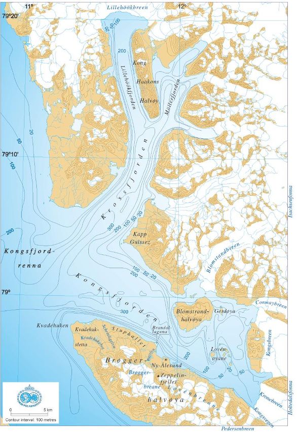
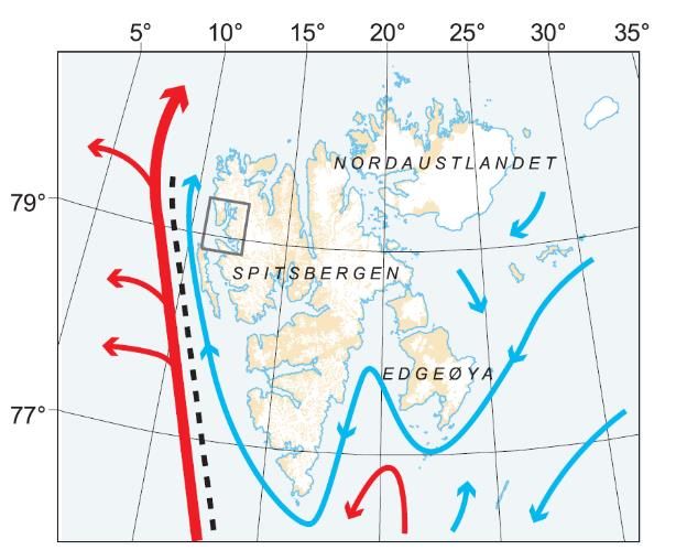
Materials and methods
__________________________________________________________________________

3 Materials and methods
3.1 Study site
 Kongsfjorden is located on the northwest coast of the Svalbard Archipelago, a group of
Arctic islands (Figure 2). It is part of the two-armed fjord system Kongsfjorden-Krossfjorden
system, which is linked to the Atlantic Ocean via a deep glacial basin, Kongsfjorddrenna
(Figure 2). The course of Kongsfjorden goes from south-east to north-west over a length of 20
km and a width of 4 to 10 km (Svendsen et al. 2002). It may be divided into several basins, an
outer basin with an average water depth of 200 – 300 m (maximal 429 m) and a distinctly
shallower inner basin with a maximal depth of 94 m (on average 50 – 60 m) (Wlodarska-
Kowalczuk and Pearson 2003).
 Oceanographic conditions of Svalbard are influenced by two major currents (Figure 2): The
West Spitsbergen Current (WSC) and the Arctic Water (ArW). The cold and fresh ArW is
flowing from the Barents Sea along the east coast of Spitsbergen to the south. At the southern
tip it merges with the WSC and heads towards the North. The WSC is the most northern
extension of the Norwegian Atlantic Current. It transports huge amounts of heat and salt along
the western shelf slope to the North. The temperature and salinity of waters west of
Spitsbergen are strongly affected by the seasonal and annual fluctuations of the WSC. The
WSC is mainly influenced by the North Atlantic Oscillation (NAO), which is the result of the
variability in the pressure ratios between the Azores High and the Icelandic Low (Cottier et al.
2005; Hop et al. 2002; Schauer et al. 2004; Svendsen et al. 2002). Further, various sources of
fresh water have a big impact on the oceanographic conditions in Kongsfjorden (Svendsen et
al. 2002). The major input of fresh water are the four tidewater glaciers draining into the fjord
(Svendsen et al. 2002). Additionally fresh water derives also from snowmelt, precipitation, river
run-off and groundwater discharge (Cottier et al. 2005). Svendsen et al. (2002) estimated the
annual discharge of fresh water to be about 1.4 km3 (annual variation up to 30 %).
 Draining of the tidewater glaciers also carries a significant amount of terrestrial sediment
(Elverhødi and Seland 1983). The sedimentation rates decline with increasing distance to the
glaciers. The rate varies between 20,000 g×m-2×a-1 at the glacier front to 1,800 –
3,800 g×m-2×a-1 in the central part of the fjord and down to 200 g×m-2×a-1 at the entrance of
the fjord (Svendsen et al. 2002).
 Considering the two different currents and the seasonal modification in oceanographic
conditions affecting Kongsfjorden it is usually addressed as a border area between Atlantic
and Arctic biogeographic zone with a precipitous gradient in sedimentation and salinity (Hop
et al. 2002). This causes a reduction in biomass and benthic community diversity in the inner

 7

Materials and methods
__________________________________________________________________________
fjord. Along this gradient a mixture of boreal and Arctic marine flora and fauna can be found
(Hop et al. 2002).

 X

 N
Figure 2: Map of Spitsbergen and the Kongsfjorden-Krossfjorden system. The black cross marks the sampling
location Brandal (78°56’52.08’’N,   11°51’9.54’’E). Upper right corner: Overview of the Spitsbergen archipelago
highlighting the major currents: West Spitsbergen Current (red line) and Arctic water (blue line). Kongsfjorden is
located within the square (adjusted from Svendsen et al. 2002).

 8

Materials and methods
__________________________________________________________________________

3.2 Shell collection and environmental data
 The cockles used for this study were caged in an enclosure on the seafloor in order to
retrieve them every year for treatment (Figure 3). Additionally water temperature and salinity
were recorded at this site.
 The position for the setup was situated near the shore in a water depth of 9 m (Brandal,
78°56’52.08’’N,  11°51’9.54’’E). The enclosure covered a field of 3 x 3 m (Figure 3). Its extent
into the sediment was about 30 cm. The sub-population of Greenland cockles contained in the
enclosure was collected in its near surroundings. On an annual basis all cockles thriving in the
enclosure were marked mechanically with a small notch from the perpendicular on ventral shell
margin up on one shell side. For this an electric underwater rotary drill (Dremel 8200 12VMax,
Racine, WI, USA) sealed in a custom-made underwater housing and equipped with one or two
cut-off wheel (Dremel cut-off wheel No. 409, Ø 24 mm, 0.6 mm thick) was used (Laudien, Brey,
and Arntz 2003). The number of individuals within the enclosure was kept stable by replacing
gathered cockles. The enclosure was cleaned from colonizing and entrapped drifting
macroalgae at least once a year.
 To continuously record water temperature and salinity a combined temperature and
conductivity logger (µS-Log540, Driesen + Kern GmbH, Bad Bramstedt, Germany) was used.
The sensors were located approximately 1.5 m away from the enclosure and about 25 cm
above the seafloor. The logger was mounted to a rod and covered with a black plastic cylinder,
which was open at the lower end. It recorded the data in intervals of 10 min from September
2009 until September 2014 (Laudien 2011, 2013). Due to a technical malfunction data from
June 2011 to September 2012 was not recorded.

 9

Materials and methods
__________________________________________________________________________

Figure 3: Enclosure (3 x 3 m) where the population of Greenland cockles was held. Exact location of the enclosure
can be seen in Figure 2. (Photo: M. Schwanitz)

3.3 Shell preparation
 In total 40 representatives individuals of S. groenlandicus were re-collected in 2012 and 10
individuals in 2014. Individuals were dissected, the shells separated from the respective soft
tissue, and thereafter cleaned with a toothbrush before air-drying. Subsequently all shells used
in this study were cross sectioned. In order to prepare a cross section along the line of
strongest growth (LSG; see Figure 1) the shell has been stabilized using a two-compounded
metal-epoxy resin (1:1 ratio; WIKO EPOXY METALL; GLUETEC, Greußheim, Germany). It
was applied on the inside and outside of the shell, following the LSG from the umbo to the
margin in a ca. two centimeters wide coat. The resin was left to dry for 12 hours at room
temperature. Thereafter the shells were cut with a circular saw bench (FKS/E; Proxxon,
Föhren, Germany) and a diamond coated cutting blade (blade: NO 28 735; Proxxon, Föhren,
Germany). The sectional surface was grinded until the growth lines became visible, utilizing a
manual grinder (Phoenix Alpha; Buehler, Düsseldorf, Germany) and abrasive paper (grain
sizes: 25 µm, 15 µm, 10 µm and 5 µm). For stability reasons the shell halves without the notch
were selected, therefore it was not possible to use always the same shell valve.

 10

Materials and methods
__________________________________________________________________________

3.4 Representativeness of individual growth
 The population structure was examined regarding general growth parameters such as the
timing of growth line deposition and growth rate.

3.4.1 Growth line deposition
 The time of growth line deposition was determined by a mark and recapture approach. In
the years 2008, 2009 and 2011 shells were labelled with calcein (Merck; Darmstadt, Germany)
following Herrmann et al. (2009) and Riascos et al. (2007). The incubation with 100 mg l-1
calcein solution took place in aerated seawater in a cold room for three hours (Figure 4). This
procedure resulted in clearly visible fluorescent lines without any mortality.
 Calcein lines were viewed in the cross sections using a fluorescence light source (Model
U-ULS100HG, Olympus, Hamburg, Germany) attached to a microscope (Research
Stereomicroscope System SZX12, Olympus, Hamburg, Germany). The shell as well as the
umbo was examined (Figure 5). Pictures were taken using a digital camera mounted to the
microscope (CCD-camera U-CMAD3 Colorview I; Olympus, Hamburg, Germany) and a
supplementary image analysis software (AnalySIS 5.0 Copyright 1986-2004; Soft Imaging
System GmbH, Olympus, Hamburg, Germany).

Figure 4: Incubation of Greenland cockles in 100 mg l-1 calcein solution. Visible are several Greenland cockles with
extended siphons. (Photo: G. Veit-Köhler)

 11

Materials and methods
__________________________________________________________________________

Figure 5: Examples for calcein lines under reflected (left hand side) and fluorescent lights (Right hand side). Green
lines visible under fluorescent lights in the umbo (top) and shell increment (bottom) are calcein lines. Positions of
calcein lines were detected by comparison with pictures taken under reflected lights.

 12

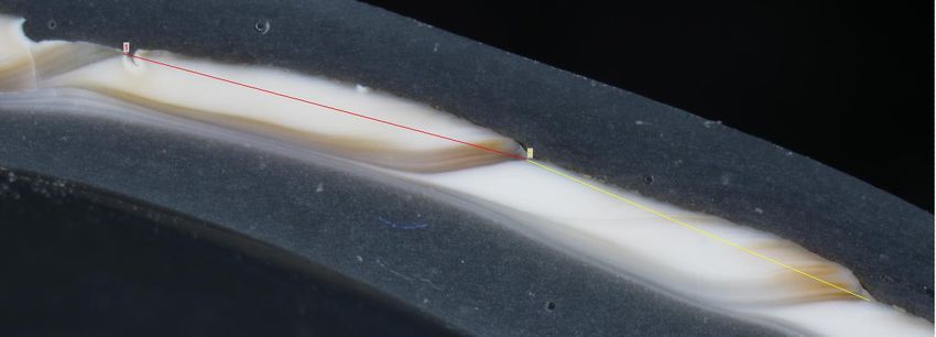
Materials and methods
__________________________________________________________________________
3.4.2 Growth rate
 For describing the growth rate of S. groenlandicus the widths of their increments were
measured. These increments represent the annual increase in shell size and allow the
modelling of a growth function.
 The measurement of increment widths was performed using a video-imaging-system (see
Section 3.4.1). The shells were fixated with periphery wax (Surgiden, Handewitt, Germany)
onto a glass-slide (76 x 26 mm) in order to achieve and maintain a parallel plane between the
camera and the cross section. Measuring started at the first dark growth line visible in the
ontogenetically youngest part of the shell. The first increment was excluded to define a clear
and unified starting point for all shells.
 An increment was defined as the distance from the end of one dark growth line to the end
of the next dark growth line in direction of growth (DOG) (Figure 6). In order to minimize
systematic errors, the means of three measurements of the same increment were calculated.
The last increment of each shell was excluded since it was still under development at time of
sampling.

Figure 6: S. groenlandicus: Measurement of the width of two increments using AnalySIS 5.0 software. Width of
increments was measured from the end of one growth line to the end of the next in direction of growth (DOG). Red
line indicates ontogenetic year one, while the yellow line indicates ontogenetic year two.

 Shell growth was modeled by fitting a von Bertalanffy growth function to the shell height-
at-age data using a nonlinear algorithm (Equation 1, von Bertalanffy 1957). The fitting process
was done iterative by minimizing the error square using the excel-solver (Microsoft® Office
2013) (Laudien et al. 2003). Main purpose was to compare the growth rates of the individuals
taken for the stable isotope analysis to the growth rates of the entire population.

 13

Materials and methods
__________________________________________________________________________

 = ∗ (1 −  (−  ( − )) Equation (1)

 With: – Shell height at time t
 – Asymptotic maximum shell height
 k – Growth constant
 t – Time in years
 t0 – Time when shell heigt was theoretically zero

3.5 Crystalline structure of the shell carbonate
 The crystalline structure of the biogenic calcium carbonate was analyzed using a Confocal
Raman microscope (CRM). To get further information on the crystalline structure shells were
also examined using a scattering electron microscope (SEM).

3.5.1 Confocal Raman microscopy
 Light interacts with molecules in three different ways. First by passing through, second by
getting absorbed and third by being scattered. The Confocal Raman microscopy is based on
the scattering of photons. Like absorption, scattering occurs when a photon hits a molecule
and promotes this molecule to a higher energetic state. Unlike absorption, the scattered
photon, which is emitted by the molecule when falling back to a lower energetic state, radiates
in a modified angle to the incoming laser. Additionally scattering does not require the incident
frequency to match the difference between the two states of the molecule. This is due to the
fact that scattering distorts (polarizes) the cloud of electrons around the nuclei, not like
absorption promoting an electron to a higher state. The energy state created by distorting the
electron cloud is determined by the frequency of the photon (Smith and Dent 2005).
 The majority of the light scatters elastically (Rayleigh scattering). Only a few photons are
scattered inelastically (Raman scattering, Figure 7). Rayleigh scattering occurs when only the
cloud of electrons is involved and no measurable energy is transferred between photon and
molecule. The scattered photon has the same frequency as the one emitted by the laser. A
Raman scattering includes an effect on the nucleus, causing energy to transfer from the photon
to the molecule (Stoke scattering). The molecule gets  promoted  from  the  ground  state  “m”  to  
a   higher   energetic   state   and   by   emitting   a   photon  falls   to   the   slightly   excited   state   “n”.   The  
scattered photon has a different frequency as the incident. This shift in energy (Stokes shift) is
molecule specific. The natural occurrence of this slightly exited state of a molecule is
determined by temperature. When irradiated with a laser it will cause an energy transfer from
 14

Materials and methods
__________________________________________________________________________
the molecule to the photon, an Anti-Stoke scattering. The change in energy state of the
molecule also matches the Stokes shift. The Confocal Raman microscope measures the
frequency differences between the laser and the scattered light and thus the Stokes shift
(Smith and Dent 2005). These measured spectra of frequency peaks are specific for each
mineral and mineral polymorph. In case of biogenic calcium carbonate it can e.g. be used to
distinguish between calcite and aragonite (e.g. Nehrke and Nouet 2011)

Figure 7: Rayleigh and Raman scattering. Raman scattering differentiated in Stokes and anti-Stokes scattering.
Energetic  ground  state  “m”  at  the  bottom,  slightly  excited  state  “n”  above it. High energetic states at the top (Smith
and Dent 2005).

 For CRM analysis the shells needed to be embedded into Araldite®, a fluid epoxy resin
(Araldite®2020, Huntsman, Bad Säckingen, Germany) since this is not so like to get burned
by the laser as the previously used metal-epoxy.
 Four shells were embedded in Araldite without further preparation (shell IDs:
27ASGkofj2012, 01-, 03-, 05ASGkofj2014). In order to get rid of the periostracum and organic
residues one shell (shell ID: 10ASGkofj2012) was previously submerged in 13 % sodium
hypochlorite-solution for 10 min. Two shells were already coated with metal-epoxy resin (see
Section 3.3) and previously cross sectioned. After removing the metal-epoxy resin from the
outer side of the shell they were embedded in Araldite (shell IDs: 17-, 25ASGkofj2014).
 Embedment of the shells with Araldite took place in a small container built from aluminium
foil. It was internally coated with a release agent (Nr. 20-8185-002, Buehler, Düsseldorf,
Germany) to prevent the Araldite from sticking to it. First the ground of the container was
covered with a thin layer of epoxy. Either the shell was put cross section downwards or as a
whole shell valve, inner side up into the container. Afterwards the shell was covered completely
with Araldite. The embedding was left to dry for 24 h. In case the entire shell was embedded
a low-speed precision saw (IsoMet, Buehler, Düsseldorf, Germany) with a 0.4 mm diamond-
 15

Materials and methods
__________________________________________________________________________
coated saw blade was utilized to cut along the LSG. Embedded cross sections were ground
using a manual grinder (Phoenix Alpha; Buehler, Düsseldorf) and abrasive paper (grain sizes:
25 µm, 15 µm, 10 µm and 5 µm) until the growth line was visible. In case the shell was already
cross sectioned it was grounded until no Araldite was covering the cross section any longer.
 For analysis a Confocal Raman microscope (alpha 300 R; WITec, Ulm, Germany) and a
monochromatic light sources with a wavelength of 488 nm and a 20 objectives (EC Epiplan,
NA = 0.4; Zeiss, Oberkochen, Germany) was used. Signals were detected using a UHTS300
ultra high throughput spectrometer (WITec GmbH, Ulm, Germany) and processed with WItec
Project FOUR (WITec GmbH, Ulm, Germany).

3.5.2 Electron microscopy
 In order to have a check for porosity in the carbonate two shell cross sections were
analyzed utilizing a scattering electron microscope (Quanta FEG 200; FEI, Oregon, USA). One
of the shells was coated with metal-epoxy (see Section 3.3). One has been embedded in
Araldite (see Section 3.5.1). SEMs produce high resolution images of a surface by
distinguishing between elastical or inelastical scattering of incident electrons. To do so sample
need to be conductive (Colliex 2008). Since the shells were not conductive they were prior to
analyzing with SEM mounted onto aluminum stubs using conductive adhesive tape and coated
with a gold/palladium layer (Sputter coater SC7640; Quorum Technologies, Lewes, United
Kingdom).

 16

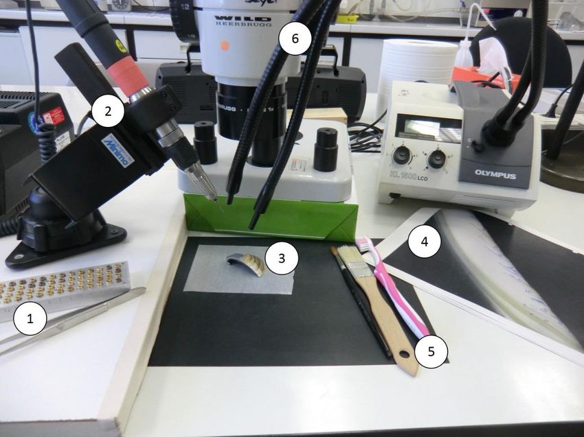
Materials and methods
__________________________________________________________________________

3.6 Stable oxygen and carbon isotopes
 Before measuring stable isotopes in biogenic calcium carbonate (CaCO3) the carbonate
samples needed to be milled from the shell. Three individuals were selected, depending on
their age and shell thickness (shell IDs: 01ASGkofj2014, 03ASGkofj2014, 06ASGkofj2014).
The δ18O  and  δ13C values of the biogenic shell carbonate were measured using an isotope
ratio mass spectrometer (IRMS). Finally they were aligned to calculated δ18O  and  δ13C values
of the shell.

3.6.1 Sampling of biogenic calcium carbonate of shells
 The sampling of the shell carbonate was carried out with a high precision drill (power pack:
Minimo C121; Rotary Handpiece: V11H; Minitor Co., Ltd., Tokyo, Japan) in combination with
a binocular microscope (WILD Heerbrugg Gais, Switzerland) and stereo microscope lighting
(KL 1500 LCD; Olympus, Hamburg, Germany).
 Initially the shells were cross sectioned as described in Section 3.3. Thereafter the epoxy
cover was removed using a cylindrical drill bit (Nr. H364E 123 010; Komet/Gebr. Brasseler
GmbH & Co. KG, Lemgo, Germany). Additionally leftover parts of the periostracum were
removed. In order to maximize the spatial sample resolution, all samples were milled (Dettman
and Lohmann 1995) manually.
 A cylindrical drill bit (Nr. H364E 123 010; Komet/Gebr. Brasseler GmbH & Co. KG, Lemgo,
Germany) was used to mill the CaCO3 samples (Figure 8). As sample region, the increments
representing the growth period from 2011 to 2013 including adjacent growth lines were chosen.
Sampling was performed in DOG from ontogenetic younger to older shell parts, parallel to the
growth lines. The first step was to create an initial-hollow in the ostracum (Figure 8). Shaping
the hollow-side, facing sampling direction, parallel to the next growth line is the most important
factor. All samples were milled in parallel lines from this side extending the sampling-hollow
towards the margin. The extracted carbonate powder was gathered by an underlying weighing
paper and successively put into sample-containers. To make sure the sampling follows the
growths pattern, adjustments to the hollow-side were made if required. During the sampling
procedure the progress was documented in high-resolution copies of the cross section images
in order to make the subsequently aligning of the samples more accurate.
 Between each sample the drill bit was cleaned by removing left over carbonate with a
toothbrush and a paintbrush. Prior to working with a new individual the drill-bit was cleaned by
placing it in an ultrasonic bath (Sonorex Super RK510; Bandelin, Berlin, Germany) for 5 min.
Cups (1 cm in diameter) held by 4 15 trays with lid, were used as sample-containers (in-house
manufacturing, Alfred-Wegener-Institut, Helmholtz-Zentrum für Polar- und Meeresforschung).

 17

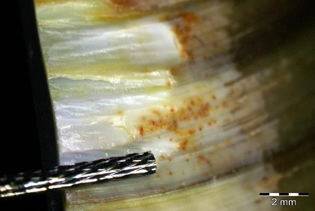
Materials and methods
__________________________________________________________________________
Before usage, all cups were first cleaned in an ultrasonic bath for 5 min, followed by rinsing
with diluted phosphoric acid.

 DOG

 500 µm

 2 mm

Figure 8: Sampling of calcium carbonate for stable isotopes analysis. Top: General set up.
1 – sample-containers, 2 – high precision drill, 3 – sample on weighing paper, 4 – high-resolution photo of the cross
section for documenting the progress, 5 – tools for cleaning the drill bit between each sample, 6 – binocular
microscope and lightning system. Bottom-left hand side: Cross section of a shell along the LSG. Red area gives
shape of the initial-hollow. Black lines indicate theoretical sampling lines. Resolution not to scale. Bottom-right hand
side: Drill bit extending the initial-hollow towards the margin.

 18

Materials and methods
__________________________________________________________________________
3.6.2 Measurement of stable oxygen and carbon isotopes
 The ratios of 18O/16O and 13C/12C were measured using an isotope ratio mass spectrometer
(IRMS). This measurement of stable isotopes is based on the fact that charged molecules are
deflected differently regarding their weight. This requires the samples to be prior transformed
from solid carbonate into CO2 by dissolving the carbonate samples with phosphoric acid
(Budzikiewicz 2005). This was carried out with an automated carbonate preparation device
(Kiel IV; Thermo Finnigan, Bremen, Germany). The CO2 was analyzed in a MAT 253 isotope
ratio mass spectrometer (Thermo Finnigan; Bremen, Germany) by ionization and separating
according to their mass-to-charge ratio. The measurements were calibrated against to the
international NBS-19   standard,   reported   in   δ-notation versus VPDB (Vienna Peedee
Belemnite) (Coplen 1994; Craig 1957) and given as parts per million. For δ18O the long-term
precision based on an internal laboratory standard measured over a one-year period was
better  than  ±0.08‰  and  better  than  ±0.06  ‰ for δ13C. For measurement 40 – 100 µg calcium
carbonate per sample were weighed in using a precision scales (Sartorius, Göttingen,
Germany).

3.6.3 Alignment of measured and calculated δ18O values
 In order to correlate the measured δ18O of the shell (δ18Oshell) with parameters measured
 18
from the environment, latter parameters needed to be converted into predicted O/16O ratios
of the shell (δ18Opredicted). Afterwards they were assigned chronological in order to align δ18Oshell
accordingly.

Calculation  of  δ18Opredicted
 The δ18Opredicted values were calculated from ambient sea temperature and salinity
measurements (see Section 3.2). First by computing the stable oxygen isotope ratio influenced
by  salinity  (δ18Os). The calculation was performed using the relationship of salinity of seawater
and  δ18Os described for Kongsfjorden by Maclachlan et al. (2007) (Equation 2):

   = (0.43   ×   ) − 14.5 Equation (2)

 With: δ18Os – Stable oxygen isotope ratio influenced by
 salinity
 Ssea – Salinity of the seawater

 19

Materials and methods
__________________________________________________________________________
 For further conversion the approach of Grossman and Ku (1986) including a small
modification (Dettman et al. 1999) was applied (Equation 3). It describes the combined
influence of seawater temperature and δ18Os, on the stable oxygen isotope ratio of biogenetic
aragonite. Verification of the crystalline structure of the shell carbonate was carried out using
confocal Raman microscopy (CRM, see Section 3.6).

   = (20.6 + 4.34 × (   − 0.27) − ) × 4.34
 Equation (3)

 With: δ18Opredicted – Predicted stable oxygen isotope ratio
 of the shell carbonate
 δ18Os – stable oxygen isotope ratio influenced by
 salinity
 Tsea – Temperature of the seawater [°C]

Alignment of δ18Opredicted and δ18Osea
 An alignment was carried out between the δ18Opredicted and δ18Osea values. The first step was
to arrange the δ18Opredicted values on a time-scale according to their recoding date. Next step
was to mark the δ18Oshell values representing the growth line. They were used as an anchor
point and aligned first, since it is known that S. groenlandicus deposits its growth line in late
summer or early fall (Ambrose et al. 2012),. Subsequently the data in between were matched
point-by-point to the   δ18Opredicted graph until the best fit was obtained (Hallmann et al. 2008;
Versteegh et al. 2012).

 20