Asphaltoberbau und extreme Temperaturen - Berichte der Bundesanstalt für Straßenwesen - Carl Ed ...
←
→
Transkription von Seiteninhalten
Wenn Ihr Browser die Seite nicht korrekt rendert, bitte, lesen Sie den Inhalt der Seite unten
Asphaltoberbau und
extreme Temperaturen

                    Berichte der
Bundesanstalt für Straßenwesen
               Straßenbau   Heft S 156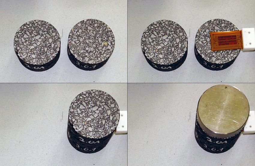
Asphaltoberbau und
extreme Temperaturen

                                                       von

                             Hartmut Johannes Beckedahl
                                           Tim Schrödter
                                          Stefan Koppers
                                         Dmytro Mansura

                           Bergische Universität Wuppertal
Lehr- und Forschungsgebiet Straßenentwurf und Straßenbau
                               Bergisches Straßenbaulabor

                                            Oscar Reutter
                                        unter Mitarbeit von
                                          Charlotte Thelen

       Wuppertal Institut für Klima, Umwelt, Energie gGmbH

                    Berichte der
Bundesanstalt für Straßenwesen
                            Straßenbau       Heft S 156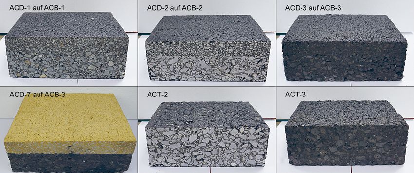
Die Bundesanstalt für Straßenwesen veröffentlicht ihre Arbeits- und Forschungs ergebnisse in der Schriftenreihe Berichte der Bundesanstalt für Straßenwesen. Die Reihe besteht aus folgenden Unterreihen: A - Allgemeines B - Brücken- und Ingenieurbau F - Fahrzeugtechnik M- Mensch und Sicherheit S - Straßenbau V - Verkehrstechnik Es wird darauf hingewiesen, dass die unter dem Namen der Verfasser veröffentlichten Berichte nicht in jedem Fall die Ansicht des Herausgebers wiedergeben. Nachdruck und photomechanische Wiedergabe, auch auszugsweise, nur mit Genehmigung der Bundesanstalt für Straßenwesen, Stabsstelle Presse und Kommunikation. Die Hefte der Schriftenreihe Berichte der Bundesanstalt für Straßenwesen können direkt bei der Carl Ed. Schünemann KG, Zweite Schlachtpforte 7, D-28195 Bremen, Telefon: (04 21) 3 69 03 - 53, bezogen werden. Über die Forschungsergebnisse und ihre Veröffentlichungen wird in der Regel in Kurzform im Informationsdienst Forschung kompakt berichtet. Dieser Dienst wird kostenlos angeboten; Interessenten wenden sich bitte an die Bundesanstalt für Straßenwesen, Stabsstelle Presse und Kommunikation. Die Berichte der Bundesanstalt für Straßenwesen (BASt) stehen zum Teil als kostenfreier Download im elektronischen BASt-Archiv ELBA zur Verfügung. https://bast.opus.hbz-nrw.de Impressum Bericht zum Forschungsprojekt 07.0276 Asphaltoberbau und extreme Temperaturen Fachbetreuung Rolf Rabe Referat Asphaltbauweisen Herausgeber Bundesanstalt für Straßenwesen Brüderstraße 53, D-51427 Bergisch Gladbach Telefon: (0 22 04) 43 - 0 Redaktion Stabsstelle Presse und Kommunikation Druck und Verlag Fachverlag NW in der Carl Ed. Schünemann KG Zweite Schlachtpforte 7, D-28195 Bremen Telefon: (04 21) 3 69 03 - 53 Telefax: (04 21) 3 69 03 - 48 www.schuenemann-verlag.de ISSN 0943-9323 ISBN 978-3-95606-603-0 Bergisch Gladbach, August 2021
3

Kurzfassung – Abstract

Asphaltoberbau und extreme Temperaturen                Asphalt pavement structures and extreme
                                                       temperatures
Analysen von Klimasimulationen des Deutschen
Wetterdienstes zur Ableitung zukünftiger Klima-        Analyses of climate simulations carried out by the
randbedingungen haben gezeigt, dass es in              German Weather Service to derive future climate
Deutschland bereits in naher Zukunft zu einer Er-      boundary conditions have shown that there will be a
wärmung kommen wird. Die Intensität der Zunahme        climatic warming in Germany in the near future. The
ist dabei regional unterschiedlich und nimmt in fer-   intensity of the increase will vary regionally and will
ner Zukunft noch einmal zu.                            increase once more in the distant future.

Um negativen Folgen der klimatischen Änderungen        In order to counteract the negative consequences
entgegenzuwirken, wurden Materialanpassungen           of these climatic changes, material adaptations
hinsichtlich der thermophysikalischen und lichttech-   with regard to the thermo-physical and photometric
nischen Materialeigenschaften bei der Konzeption       material properties were implemented in the design
und Herstellung klimaoptimierter Asphalte umge-        and production of climate-optimised asphalts. An
setzt. Eine Optimierung der lichttechnischen Eigen-    optimisation of the photometric properties was
schaften wurde durch die Verwendung heller Ge-         achieved by using light-colored aggregates
steinskörnungen (Quarzit) und von synthetischem        (quartzite) and synthetic binders with pigments.
Bindemittel mit Pigmenten erzielt. Bezüglich der       Regarding the thermo-physical properties, asphalt
thermophysikalischen Eigenschaften wurden As-          mixes with increased (quartzite, limestone) and
phaltmischgüter mit erhöhter (Quarzit, Kalkstein)      reduced (electro-furnace slag) thermal conductivity
und verringerter Wärmeleitfähigkeit (EO-Schlacke)      were designed for all asphalt layers.
für alle Asphaltschichten konzipiert.
                                                       Radiation reflectance and thermo-physical material
An Probekörpern der konzipierten Asphaltmischgü-       properties were measured on test specimens of the
ter wurden die Strahlungsreflexionsgrade sowie die     asphalt mixes designed. Subsequently, a practical
thermophysikalischen Materialeigenschaften mes-        thermal stressing in the laboratory on 24cm thick
stechnisch ermittelt. Anschließend fand eine praxis-   asphalt superstructures in a test facility for the
gerechte thermische Beanspruchung im Laboratori-       simulation of global radiation took place. Tem-
um an 24 cm dicken Asphaltaufbauten in einer Ver-      perature gradients were determined by measure-
suchsanlage zur Simulation der Globalstrahlung         ments at different depths. In addition, a simplified
statt. Hierbei wurden Temperaturgradienten durch       one-dimensional finite element model was created
Messungen in verschiedenen Tiefen ermittelt. Zu-       on which sensitivity analyses of thermo-physical
sätzlich wurde ein vereinfachtes eindimensionales      properties and comparisons with the laboratory
Finite-Elemente-Modell erstellt, an dem Sensitivi-     results were carried out.
tätsanalysen zu thermophysikalischen Eigenschaf-
ten sowie Vergleiche zu den Laborergebnissen           As expected, the variants with light-colored surface
durchgeführt wurden.                                   course and aggregates with higher thermal con-
                                                       ductivity achieved the lowest heating in the asphalt
Erwartungsgemäß erreichten die Varianten mit hel-      pavement. The temperature rise in the asphalt base
ler Deckschicht und Gesteinskörnung mit höherer        course depends on the thermal conductivity of the
Wärmeleitfähigkeit die geringsten Erwärmungen im       asphalt binder layer and the asphalt base course.
Asphaltoberbau. Der Temperaturanstieg in der ATS
ist dabei abhängig von den Wärmeleitfähigkeiten        To conclude, asphalt and binder tests were
der ABS und ATS.                                       successfully carried out to determine and assess
                                                       the performance of the designed asphalts.
Abschließend wurden Asphalt- und Bindemittelprü-
fungen zur Bestimmung und Beurteilung der Perfor-
mance der konzipierten Asphalte durchgeführt.
4
Summary out by the German Weather Service and a catalogue
of climate indices for individual and consecutive
days was compiled, which is based on high-
resolution data of an ensemble of regional climate
Asphalt pavement structures and extreme
models for Germany and the adjacent river basins.
temperatures
Especially for this research project, different climate
elements were combined, which, according to first
estimates, leads to a maximum warming of an
asphalt package.
1 Initial situation and objectives
of the project The analysis for the derivation of future climate
boundary conditions shows that in the entire BRD
In research [1-4], which takes into account the area for the emission scenarios RCP4.5 and
projected climate change when dimensioning road RCP8.5 warming will already occur in the near
pavements, it was shown that the durability of road future (time slice 2031 to 2060). The intensity of the
pavements is significantly influenced by climatic increase differs in some regions and will increase
changes (e.g. increase in the frequency and again in the distant future (time slice 2071 to 2100).
intensity of heat waves). Among other things,
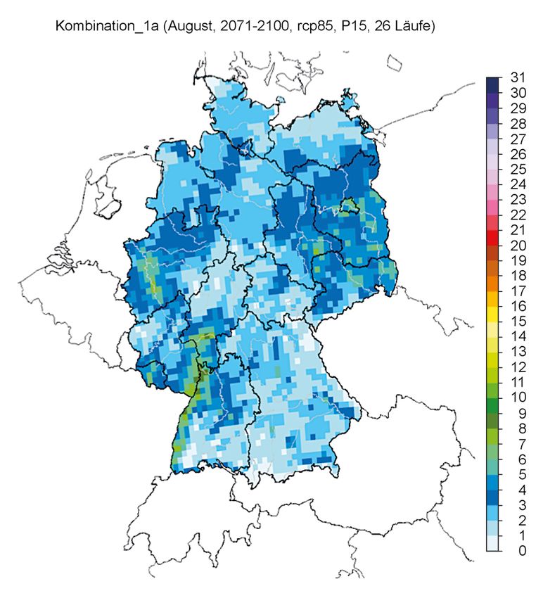
sensitivity analyses have shown that the service life Extreme climatic events such as the combination 1
of asphalt base layers is shortened due to the (heat period with tropical nights) occur more
current standardised asphalt pavement designs, frequently, but their intensity varies greatly from
taking into account the projected climate change. In region to region. Frequently, strong changes,
addition, the more frequent occurrence of high especially with regard to daily maximum
temperatures increases or accelerates the growth temperatures and the intensity of periods, can be
of permanent deformations, in some cases observed in the east, on the Upper and Lower
significantly. Rhine, in the Rhine-Main area and in Bavaria. In
terms of changes in night-time temperature
This research project follows earlier research work. changes, the north and the coastal region are most
The aim is to make reliable statements regarding affected.
the possibilities of compensation through material
optimisations on the effects of the projected climate The effects of climate change on the performance of
change. To this end, existing asphalt types and asphalt and the resulting consequences for future
grades are being redesigned with regard to their road construction are mainly limited to extreme
thermo-physical properties within the framework of temperatures (in the sense of high asphalt
this research project. Albedo is also taken into temperatures). As the probability of very low
account as a measure of the reflection of thermal temperatures due to global warming will be lower in
radiation. the future, but their occurrence cannot be excluded,
the possible widening of the temperature range
The aim of the research project is to influence the between maximum and minimum asphalt tem-
performance parameters of asphalt by a targeted peratures must also be taken into account.
material adaptation in such a way that the effects of
climate change on service life and maintenance In order to counteract the negative consequences
intervals can be kept as low as possible. of climatic changes, material adaptations with
regard to the thermo-physical and photometric
material properties, which have been implemented
in the design and manufacture of climate-optimised
2 Research methodology and asphalts, can be purposeful. An optimisation of the
results light-engineering material properties was achieved
by using light-colored aggregates (quartzite) and
In order to derive future climatic boundary conditions synthetic binder with pigments. Regarding the
and their effects on the temperature development in thermo-physical material properties, asphalt mixes
an asphalt road surface, different climatic elements with increased (quartzite and limestone) and
and climatological events have to be analysed first. reduced (EO slag) thermal conductivity were
For this purpose, climate simulations were carried designed for all asphalt layers. Laboratory tests
5
Asphalt capacity of a material. The metrological deter-
Variant Aggregates Binder Miscellaneous
mix type mination of thermo-physical material properties was
ACD-1 Diabase PmB - carried out with a THB measuring instrument on
flat-ground marble specimens with a diameter of
ACD-2 Quartzite PmB -
100mm.
AC 8 D ACD-3 EO slag PmB -
ACD-7 Quartzite SynB Pigments As expected, the lowest thermal conductivity (1.23
ACD-9 EO slag SynB Pigments to 1.29 W/(m*K)) was determined for the variants
with EO slag. The cover layers with quartzite as an
ACB-1 Diabase PmB
aggregate are much higher (2.60 to 3.09 W/(m*K))
AC 16 B ACB-2 Limestone PmB
and the reference variants with diabase are in
ACB-3 EO slag PmB between (1.59 to 1.89 W/(m*K)). For the layers
ACT-1 Diabase StBB with more voids, measurements were only possible
AC 22 T ACT-2 Limestone StBB to a limited extent (asphalt binder course) or not at
all (asphalt base course).
ACT-3 EO slag StBB
Tab. 1: Mix designs for asphalt wearing courses, asphalt binder The practice-oriented thermal stressing of the
courses and asphalt base courses asphalt specimens took place in the laboratory in a
test facility (irradiation stand) built for this research
were carried out on both the individual layers and
project to simulate global radiation. In the irradiation
combinations of these layers. A selection of the
stand, asphalt structures with a thickness of 24cm
asphalt mixes designed for asphalt wearing courses,
were irradiated with sunlight lamps and the
asphalt binder courses and asphalt base courses is
temperature gradients were recorded by tem-
shown in table 1.
perature measurements at various depths. The
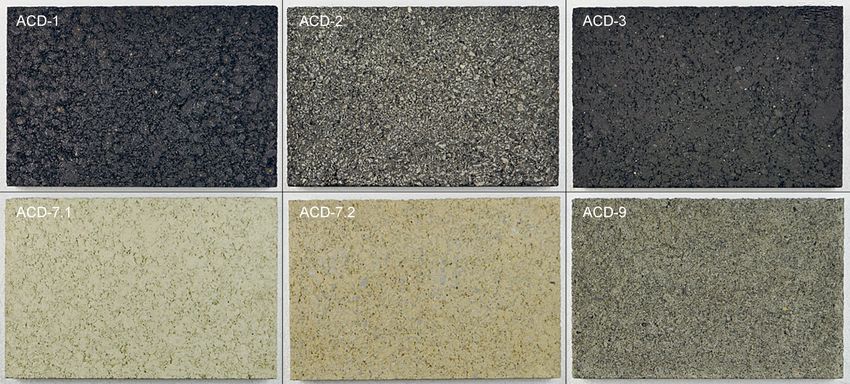
The photometric material properties of an asphalt asphalt superstructures were composed of different
wearing course (ADS) can be improved by using a combinations of the designed asphaltic pavements.
light-colored aggregate within the asphalt or as a In the case of the practice-oriented thermal stress,
gritting material on its surface. The use of synthetic the influence of different thermo-physical asphalt
binders, which can be lightened with pigments, properties was primarily investigated. The reflectivity
offers further optimisation potential. Within the was only dependent on the color of the binder film
scope of this research project, the radiation on the surface, as no surface treatment was applied.
reflection coefficients of six asphalt surface layer
The greatest temperature reduction in the bonded
variants were determined by measurement. The
superstructure was achieved by the variant with a
radiation reflectance indicates the proportion of
light and heat-conducting asphalt surface layer
radiation in the entire solar spectrum that is reflected
(quartzite and synthetic binder with pigments) on an
by the asphalt.
asphalt binder and asphalt base layer with low
The lowest (0.042) and the highest (0.484) radiation thermal conductivity (EO slag). The other variants
reflectance are the surface untreated asphalt with a light-colored surface course and aggregates
wearing courses with PmB and SynB with pigments. with higher thermal conductivity also lead to
These surfaces correspond to a freshly produced significantly less heating in the bonded super-
asphalt surface layer and have a continuous binder structure. The temperature increase in the asphalt
film, just like the surfaces of the asphalt specimens base layer (ATS) depends on the thermal con-
in the irradiation booth. The measurement results ductivity of the asphalt binder course (ABS) and the
could therefore be used for the application of the ATS.
laboratory results in the model. With a value of
0.125, the asphalt surface layer variant with quartzite The asphalt variants with dark surface layer, which
as an aggregate and glass break blasted surface were optimised in terms of their thermo-physical
performs best in the concepts with PmB. material properties, did not lead to any reduction in
the heat in the ADS after 27 hours. In the lower
The thermo-physical properties of a material have third of the ATS, only slightly lower temperature
a significant influence on heat conduction and differences could be measured in three variants
storage. They are influenced, among other things, compared to the reference variant. It must be taken
by the density, thermal conductivity and heat into account that no surface treatment was carried
6

out on the variants with a dark surface layer and        by conventional binder tests (PEN, EP RuK, BPFr,
their radiation reflectance therefore corresponds to     RE) and the BTS method.
that of a freshly applied asphalt surface layer.
                                                         The resistance to permanent deformation was
In order to analyse the effect of the thermo-physical    determined using two different test methods, the
and photometric asphalt properties, a simplified         cyclic compression test according to DIN EN 12697-
one-dimensional finite element model for heat            25 [5] and the track formation test according to TP
transfer was created. A sensitivity analysis on the      Asphalt StB Part 22 [6]. The resistance to permanent
single-layer model allowed qualitative statements to     deformation was determined in both tests under
be made on the influence of the increase or reduction    otherwise identical conditions. An adjustment of the
in thermal conductivity, specifically on heat capacity   test temperatures to the temperatures to be
and density on temperature development.                  expected due to the thermo-physical and light-
                                                         technical material properties was not carried out in
The multi-layer model, which corresponds to a            the test arrangements. The statements are therefore
structure of the load class Bk10 according to the        only relative. The effects of the temperatures on the
guidelines for the standardisation of pavement           development of the permanent deformations of the
structures of traffic areas (RStO 12), was first         asphalts tested here can only be estimated by
calibrated in several steps and then used to verify      means of theoretically based prognosis models with
the results of the practical thermal stress in the       which the thermo-physical and photometric material
laboratory. For this purpose, the asphalt pavements      properties can also be represented.
used in the laboratory were simulated with the
corresponding thermo-physical and photometric            The stiffness was determined as a function of
material properties. Based on the measured global        frequency and temperature. As asphalt stiffness
radiation values during the tests in the irradiation     based on a frequency of 10Hz are usually used for
booth, a constant radiation of 600 W/m² was applied.     stress and strain calculations and performance
The initial and ambient temperature was set at           forecasts, the summarising evaluations are also
20°C and a heat transfer coefficient for still air.      based on this frequency.

The comparison of the model calculations with the        The stiffnesses for the asphalt surface layer variants
laboratory results at a depth of 20mm (middle of the     at high temperatures range from relatively high
asphalt surface layer) shows a higher agreement          stiffnesses for ACD-3 and ACD-1, through
for the test series with darker asphalt surface layer    moderately high stiffnesses for ACD-9 and ACD-2,
(Δ = 5.7 K) compared to those with light asphalt         to the lowest stiffnesses for ACD-7. At low
surface layer (Δ = 15.8 K). At a depth of 220mm          temperatures, ACD-9, ACD-7 and ACD-3 are at a
(lower third asphalt base layer) the differences are     high stiffness level and ACD-1 and ACD-2 are at a
smaller. The test series with a dark asphalt surface     relatively low stiffness level. The stiffnesses for the
layer exceed the laboratory results (Δ = 5.2 K),         asphalt binder course variants do not differ
those with a lighter one fall short of these (Δ = 4.5    significantly at high and low temperatures. For the
K). The reasons for this are probably the higher         asphalt base layer variants, hardly any differences
ambient temperature despite air conditioning in the      can be detected at high temperatures. At low
laboratory, an excessive reduction in the amount of      temperatures, the stiffnesses for ACT-3 are higher
radiation due to the degree of reflection in the model   than for ACT-1 and ACT-2. In summary, only ACD
and the assumptions made for the thermo-physical         variants show significant differences in the
material properties for the asphalt binder and           temperature dependent stiffnesses.
asphalt base layer due to the problems described.
                                                         Based on the performance tests for resistance to
Asphalt and binder tests were carried out to test and    permanent deformation of asphalt concrete wearing
assess the performance of the designed asphalts.         courses, tested with the cyclic compression test
The stiffness and fatigue behavior were investigated     according to DIN EN 12697-25 [5], the ACD-9
by means of the indirect tensile test, the deformation   variant behaves most favorably at 50 °C test
behavior at high temperatures by means of the            temperature, independent of the test method used.
cyclic compression test and the track formation test,    In the ranking list, the variants ACD-3 and ACD-1 or
and the low temperature behavior by means of             ACD-1 and ACD-3 follow, up to ACD-2 and ACD-7.
cooling and tensile tests. The binders were analysed     Due to the stiffnesses determined, the very good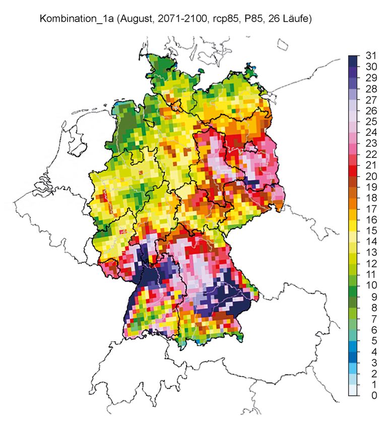
7

performance in the field of permanent deformation          volumetric binder content of the ACD-2 and ACD-3
of variant ACD-9 can be described as unusual.              variants is slightly lower than that of ACD-9. The
                                                           information on both volumetric binder content and
For the asphalt concrete binder course, the variants       the stiffness at low temperatures does not provide
rank from ACB-1, ACB-3 to ACB-2 from favorable to          any information on the low temperature behavior.
less favorable, whereby ACB-2 would have to be
classified as equivalent or even slightly more             Apart from the material adaptations investigated
favorable than variant ACB-3 in the long term due to       here, the possibilities for mix optimisation that are
the lower creep rate at the end of the test. Here, too,    already common today remain. In the publications
one variant, ACB-1, shows a considerably more              [8-10] it could be shown that the choice of binder
favorable behavior with respect to permanent               alone makes it possible to significantly influence the
deformations than the other two variants, although         performance properties of resistance to permanent
the stiffnesses at high temperatures hardly differ.        deformation, fatigue resistance and resistance to
                                                           cooling with regard to longer service lives. These
Based on the performance tests for fatigue                 test results were obtained under otherwise identical
resistance, the ACB-1, ACB-2 and ACB-3 variants            boundary conditions such as layer thickness, traffic
perform almost equally well. In contrast, the tested       and climate compared to the standard solutions. If
variants ACT-2 and ACT-3 show a significant                the above-mentioned approaches to asphalt design
difference. The variant ACT-3 shows a significantly        are combined with the usual mix optimisation,
higher resistance to fatigue in the range of the initial   including, for example, binders not yet included as
elastic strain of εel,Anf < 0.1‰ or allows significantly   standard in the TL Asphalt-StB, such as high
higher numbers of load cycles until cracking than          polymer modified bitumen (PmB H), the negative
the variant ACT-2. Since the fatigue strength is           consequences of extreme temperatures on the
tested at a temperature of 20°C, the service life due      performance behavior of asphalt can be successfully
to fatigue in an overall construction is very dependent    counteracted in any case.
on the stiffness gradients of the construction. As a
result of relatively high temperatures in the structure    As it was not part of the task catalogue of this
under consideration, the layer stiffnesses are             research project to test such asphalt combinations
                                                           by means of mix optimisation, nor to carry out
reduced and the tensile strains at the underside of
                                                           performance prognoses, a follow-up research pro-
the asphalt layer under consideration become
                                                           ject should be set up. In this project, the above-
greater for the same load. With increasing tensile
                                                           mentioned approaches to asphalt design (heat
strain at the underside, however, the service life
                                                           storage, heat dissipation and brightened surface) in
decreases. Thus, the resistance to fatigue is a
                                                           combination with high-performance binders will
performance parameter but is not sufficient to
                                                           have to be investigated by incorporating forecasts
determine the service life of asphalt structures.
                                                           of performance developments of an optimisation.
Low temperature performance is an important per-
                                                           Based on the results of this research project, a
formance property, particularly in asphalt wearing
                                                           further research project could also investigate the
courses. According to the test methods uniaxial
                                                           effects of the changed climatic boundary conditions
tensile test and cooling test according to TP Asphalt
                                                           on the service life of asphalt constructions. With the
StB part 46 A [7], the asphalt surface layer variants
                                                           help of dimensioning calculations, the effects of the
ACD-7 and ACD-9 perform worst. The variants
                                                           changed climatic conditions on the service life of
ACD-1, ACD-2 and ACD-3 are to be evaluated as
                                                           conventional asphalt constructions on the one hand
relatively equal with regard to the low temperature
                                                           and climate-optimised asphalts on the other hand
behavior. It should be briefly mentioned here that
                                                           could be analysed. Thus, the questions regarding a
the low temperature properties of asphalt deteriorate
                                                           possible shortening of the service life due to climate
with decreasing binder film thickness. The binder
                                                           changes or an extension of the service life by
content expressed in % by volume gives an indi-
                                                           asphalt mixes adapted to the climate changes could
cation of this, unless the aggregates are porous.          be clarified.
Looking at the binder content of the asphalt wearing
course variants, the synthetic binder variants have        In addition to the pure adaptation of asphalt mixes
the lowest and the highest volumetric binder content       to the extreme temperatures caused by climate
(ACD-7). The ACD-1 variant has a slightly higher           change, the impact of climate change on asphalt
volumetric binder content than ACD-7, while the            performance can also be reduced by transport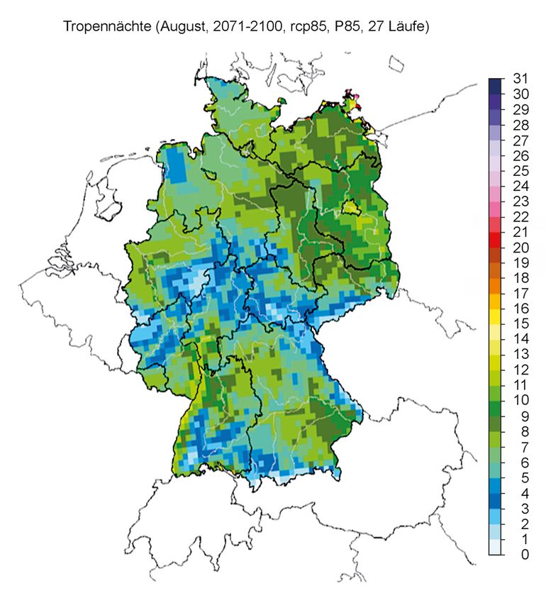
8

policy decisions. In this context, the limitation of
axle loads, by avoiding overloading with the help of
vehicle technology (smart trucks), and the
distribution of the vehicle mass over a larger area
(reduction of the stress transmitted from the tire to
the road surface), by increasing the number of axles
per vehicle or by using tires that are less damaging
to the road surface, are particularly worth mentioning.
Political control would be possible through an
architecture of tolls geared to this. Such measures
could possibly reduce the effects of extreme
temperatures on asphalt performance as an
alternative or in combination with construction
technology or optimisation of construction material
components.

In conclusion, it should be noted that the search for
solutions is not a distant future problem but must be
implemented quickly. If one assumes that asphalt
base layers are currently estimated to have an
average service life of 50 years, new asphalt base
layers built for example for major renovations are
already today in the near future (time slice 2031 to
2060) and even beyond. It is therefore necessary to
set future temperatures for current dimensioning of
pavement structures.
9
Inhalt
Abkürzungen . . . . . . . . . . . . . . . . . . . . . . . . . 11 4.2 Vorbereitungen und Vorgehensweise
bei der Analyse . . . . . . . . . . . . . . . . . . . 26
1 Einleitung . . . . . . . . . . . . . . . . . . . . . . . 13 4.3 Analyse der Klimadaten . . . . . . . . . . . . 27
2 Treibhausgasemissionen in 5 Konzeption und Herstellung
Deutschland und weltweit . . . . . . . . . 14 klimaoptimierter Asphalte . . . . . . . . . 34
2.1 Betrachtung von Vergangenheit 5.1 Ansprache thermophysikalischer
und Gegenwart . . . . . . . . . . . . . . . . . . . 14 und lichttechnischer Asphalt-
eigenschaften . . . . . . . . . . . . . . . . . . . . 34
2.1.1 Fossile Kohlenstoffdioxidemissionen . . 14
5.2 Asphaltmischgutkonzeptionen . . . . . . . 35
2.2 Typen von Zukunftsszenarien . . . . . . . . 15
2.2.1 Einführung zum fünften Sachstands-
6 Modell zur Wirkungsweise
bericht (AR5) des IPCC (Entstehung,
der thermophysikalischen
Zeitraum, Aufbau) . . . . . . . . . . . . . . . . . 15
Asphalteigenschaften . . . . . . . . . . . . . 36
2.2.2 Einführung zum Emission Gap
6.1 Numerische Modellbeschreibung . . . . . 36
Report (EGR19) . . . . . . . . . . . . . . . . . . 16
6.2 Ergebnisse . . . . . . . . . . . . . . . . . . . . . . 40
2.3 Betrachtung der Zukunft . . . . . . . . . . . . 17
2.3.1 Aussagen im fünften Sachstands- 7 Thermophysikalische und licht-
bericht des IPCC . . . . . . . . . . . . . . . . . . 17 technische Asphalteigenschaften . . . 44
2.3.2 Aussagen im Emission Gap Report 7.1 Thermophysikalische Eigenschaften . . 44
2019 . . . . . . . . . . . . . . . . . . . . . . . . . . . 18
7.1.1 Prüfverfahren . . . . . . . . . . . . . . . . . . . . 44
2.4 Übersicht der gesamten Treibhaus-
gas- und Kohlendioxidemissionen . . . . 19 7.1.2 Ergebnisse . . . . . . . . . . . . . . . . . . . . . . 45
7.2 Lichttechnische Eigenschaften . . . . . . . 47
3 Klimamodellierung und 7.2.1 Prüfverfahren . . . . . . . . . . . . . . . . . . . . 48
Asphalteigenschaften . . . . . . . . . . . . . 20
7.2.2 Ergebnisse . . . . . . . . . . . . . . . . . . . . . . 48
3.1 Klimamodellierung . . . . . . . . . . . . . . . . . 20
7.3 Praxisgerechte thermische
3.1.1 Globalmodelle . . . . . . . . . . . . . . . . . . . . 20 Beanspruchung im Laboratorium . . . . . 49
3.1.2 Regionale Klimamodelle . . . . . . . . . . . . 21 7.3.1 Bestrahlungsstand und
3.2 Mögliche zukünftige Klima- Vorbereitungen . . . . . . . . . . . . . . . . . . . 49
änderungen in Deutschland . . . . . . . . . 21 7.3.2 Ergebnisse . . . . . . . . . . . . . . . . . . . . . . 50
3.2.1 Auswirkungen auf den Asphalt- 7.4 Modellanwendung der Labor-
oberbau . . . . . . . . . . . . . . . . . . . . . . . . . 22 ergebnisse . . . . . . . . . . . . . . . . . . . . . . . 55
3.3 Materialeigenschaften von Asphalt . . . . 22
8 Konventionelle und performance-
orientierte Asphalt- und Binde-
4 Ableitung zukünftiger Klimarand-
mittelprüfungen . . . . . . . . . . . . . . . . . . 58
bedingungen . . . . . . . . . . . . . . . . . . . . 23
8.1 Bindemittelprüfungen . . . . . . . . . . . . . . 58
4.1 Auswahl von Klimaelementen und
Berechnung von Klimaindizes . . . . . . . . 23 8.2 Asphaltprüfungen . . . . . . . . . . . . . . . . . 5810 8.2.1 Druckschwellversuch . . . . . . . . . . . . . . 58 8.2.2 Spurbildungsversuch . . . . . . . . . . . . . . . 59 8.2.3 Spaltzug-Schwellversuch . . . . . . . . . . . 59 8.2.4 Kälteeigenschaften . . . . . . . . . . . . . . . . 62 9 Zusammenfassung . . . . . . . . . . . . . . . 63 Literatur . . . . . . . . . . . . . . . . . . . . . . . . . . . . . 68 Bilder . . . . . . . . . . . . . . . . . . . . . . . . . . . . . . . 72 Tabellen . . . . . . . . . . . . . . . . . . . . . . . . . . . . . 75 Die Anhänge zum Bericht sind im elektronischen BASt-Archiv ELBA unter https://bast.opus.hbz-nrw. de abrufbar.
11
Abkürzungen
ACB Asphaltbeton Binderschicht DIN EN Deutsches Institut für Normung
(DIN), Übernahme einer Euro-
ACD Asphaltbeton Deckschicht päischen Norm (EN)
ACT Asphaltbeton Tragschicht
DWD Deutscher Wetterdienst
AFOLU Agriculture, Forestry and Other
EC-EARTH European Centre – Earth
Land Use
System model
ALADIN Aire Limitée Adaptation dynamique
ECHAM European Center Hamburg
Développement InterNational
Model, Akronym aus ECMWF
ALARO Kombiniertes Model aus ALADIN und Hamburg
und AROME
ECMWF European Centre for Medium
AROME Application de la Recherche à Range Weather Forecasting
l’Opérationnel à Meso-Echelle
EDGAR Electronic Data Gathering,
AR5 IPCC Assessment Report 5 Analysis, and Retrieval
BAU Business as usual EGR Emission Gap Reports
BMVI Bundesministerium für Verkehr EOS/EO-Schlacke Elektroofenschlacke
und digitale Infrastruktur
EP RuK Erweichungspunkt Ring- und
BPFr Brechpunkt nach Fraaß Kugel
BRD Bundesrepublik Deutschland ESM Earth System Model
BTSV Bitumen-Typisierungs-Schnellver- EU Europäische Union
fahren
EURO-CORDEX Coordinated Downscaling Ex-
BTU Brandenburgische Technische periment – European Domain
Universität Cottbus-Senftenberg
FOLU Forstwirtschaft und andere
CanESM2 Canadian Earth System Model,
Landnutzung
Generation 2
GCM Global Climate Model, oder
CLINO CLINO-Periode (CLINO = climate
auch General Circulation
normal = Normalperiode)
Model
CMIP5 Climate Model Intercomparison
HadGEM2-ES Hadley Centre Global Environ-
Project, Phase 5
ment Model 2 – Earth System
CNRM Centre National de Recherches
HIRHAM Dynamisches Regionales
Météorologiques
Klimamodell des Dänischen
CNRM-CM5 Centre National de Recherches Meteorologischen Instituts,
Météorologiques – Climate Model, Kombination der Modelle
Version 5 HIRLAM und ECHAM
COSMO-CLM Consortium for Small Scale Model- HIRLAM High Resolution Limited Area
ling model in Climate Mode, auch Model
CCLM genannt
HYRAS Hydrologische Rasterdaten
DIN Deutsches Institut für Normung sätze12
IPCC Intergovernmental Panel on ReKliEs-De Regionale Klimaprojektionen
Climate Change Ensemble für Deutschland
IPSL-CM5A Institute Pierre Simon Laplace REMO dynamisches Regional-Modell
– Climate Model, Version 5A
RStO Richtlinien für die Standardisie-
KLIWAS Forschungsprogramm Klima, rung des Oberbaus von Ver-
Wasser, Schifffahrt kehrsflächen
Kombi1 PeriH + NachtT SMA Splittmastixasphalt
Kombi2 PeriH + NachtW SRES Special Report on Emissions
Scenarios
Kombi3 PeriW + NachtW
StbB Straßenbaubitumen
LULUCF Land Use, Land-Use Change and
Forestry SynB synthetisches Bindemittel
MA Gussasphalt TagH heiße Tage
MIROC5 Model for Interdisciplinary TagS Sommertage
Research on Climate, Version 5
TagW warme Tage
MPI-ESM Earth System Model des TAS mittlere bodennahe Lufttempe-
Max-Planck-Institutes ratur
MPI-M Hamburger Max-Planck-Institut für THB Transient Hot Bridge
Meteorologie
THG-Emissionen Treibhausgasemissionen
NachtT Topennächte
Tmax Tageshöchsttemperatur
NachtW warme Nächte
Tmin Tagestiefsttemperatur
NDC National Determined Contribution
TP Asphalt-StB Technische Prüfvorschriften für
NorESM Norwegian Earth System Model Asphalt
PEN Nadelpenetration UBA Umweltbundesamt
PeriH Hitzeperiode UN United Nations
PeriW Wärmeperiode UNEP United Nations Environment
Programme
PmB polymermodifiziertes Bindemittel
WRF Weather Research and
RACMO Regional Atmospheric Climate Forecast Model
Model
RCA Rossby Centre regional
atmospheric model
RCM Regional Climate Model
RCP Representative Concentration
Pathway
RDO Asphalt Richtlinien für die rechnerische
Dimensionierung des Oberbaus
von Verkehrsflächen mit Asphalt-
deckschicht13
1 Einleitung er aller Asphaltschichten verkürzt. An der Unterseite
der Asphalttragschichten erhöhen sich infolge tem-
In Forschungsarbeiten [1–4], die den projizierten peraturbedingter Steifigkeitsminderungen der Ge-
Klimawandel bei der Dimensionierung von Straßen- samtkonstruktion die Zugdehnungen und damit die
befestigungen berücksichtigen, konnte gezeigt wer- Ermüdungsschädigung. Außerdem werden durch
den, dass die Dauerhaftigkeit von Straßenbefesti- die Auswirkungen höherer Temperaturen die Schä-
gungen durch klimatische Veränderungen (z. B. Zu- digungen der Asphaltdecke in Form von bleibenden
nahme der Häufigkeit und Intensität von Hitzewel- Verformungen zunehmen. Maßnahmen der Straße-
len) deutlich beeinflusst wird. Unter anderem konn- nerhaltung müssten somit häufiger durchgeführt
te anhand von Sensitivitätsanalysen gezeigt wer- werden. Neben den steigenden Erhaltungskosten
den, dass sich bei den derzeitigen standardisierten würde dies auch zu höheren Beeinträchtigungen für
Asphaltoberbaukonstruktionen, unter Berücksichti- Straßennutzer durch mangelnden Fahrkomfort und/
gung des projizierten Klimawandels, die Nutzungs- oder Verkehrsstaus infolge von Baumaßnahmen
dauer der Asphalttragschichten verkürzt. Darüber sowie gegebenenfalls zu eingeschränkter Verkehrs-
hinaus wird durch das häufigere Auftreten hoher sicherheit durch Aquaplaning führen.
Temperaturen der Zuwachs an bleibenden Verfor-
Eine Neukonzeption der Asphalte für Deck-, Binder-
mungen teilweise deutlich erhöht bzw. beschleu-
und Tragschichten hinsichtlich ihrer thermophysika-
nigt. Durch die Annahme veränderter Materialpara-
lischen und Performance-Eigenschaften soll dazu
meter wurde auf theoretische Weise gezeigt, dass
führen, geplante Nutzungsdauern von Asphaltober-
durch Änderungen von Asphaltmischgutrezepturen
bauten trotz der zu erwartenden Auswirkungen des
negative Auswirkungen des Klimawandels auf die
projizierten Klimawandels, wie etwa häufigeren
Nutzungsdauern und Erhaltungszyklen kompensie-
und/oder längeren Perioden mit extremer Hitze,
ren werden können.
einhalten zu können.
Die Ergebnisse der Sensitivitätsanalysen sind theo-
Um auszuschließen, dass sich die Asphalteigen-
retischer Natur und wurden nicht durch Performan-
schaften der im Forschungsvorhaben für extreme
ce-Prüfungen an dafür konzipierten Asphalten veri-
(hohe) Temperaturen thermophysikalisch optimier-
fiziert. Dieses Forschungsprojekt schließt sich in-
ten Asphalte für Deck-, Binder- und Tragschicht hin-
haltlich früheren Forschungsarbeiten an. Es sollen
sichtlich des Verhaltens bei niedrigen Temperaturen
belastbare Aussagen hinsichtlich der Kompensati-
mehr als vertretbar verschlechtern, werden diese
onsmöglichkeiten durch Materialoptimierungen auf
nicht nur im Hinblick auf ihr irreversibles Verfor-
die Auswirkungen des projizierten Klimawandels
mungsverhalten und ihrer Materialkennwerte ge-
getroffen werden. Dazu werden im Rahmen dieses
mäß den Richtlinien für die rechnerische Dimensio-
Forschungsprojektes bestehende Asphaltsorten
nierung des Oberbaus von Verkehrsflächen mit As-
und -arten hinsichtlich ihrer thermophysikalischen
phaltdeckschicht (RDO Asphalt) [5] geprüft, son-
Eigenschaften neu konzipiert. Ebenso findet die Al-
dern auch bezüglich ihres Verhaltens bei tiefen
bedo, als Maß der Reflexion thermischer Strahlung,
Temperaturen. Dies ist deshalb erforderlich, weil bei
Berücksichtigung. Durch eine gezielte Erhöhung
Standardasphalten ein Zuwachs des Widerstandes
der Albedo, die ein höheres Reflexionsvermögen
gegen bleibende Verformungen mit einer Verminde-
gegenüber Wärmestrahlung bewirkt, soll die Resis-
rung des Widerstandes gegen tiefe Temperaturen
tenz gegen bleibende Verformungen bei steigender
einhergeht. Zudem werden die konzipierten Asphal-
Häufigkeit sehr hoher Tageshöchsttemperaturen
te mit einer Referenzvariante verglichen. Somit kön-
verbessert werden.
nen abschließend Aussagen zur Anwendung der
Ziel des Forschungsprojektes ist es, durch eine ge- gegen extreme Temperaturen widerstandsfähig
zielte Materialadaption die Performanceparameter konzipierten Asphalte getroffen werden.
von Asphalt so zu beeinflussen, dass die Auswir-
kungen des Klimawandels auf Nutzungsdauer und
Erhaltungsintervalle so gering wie möglich gehalten
werden können.
Ohne eine Anpassung der verwendeten Materialien
im Asphaltoberbau an den projizierten Klimawandel
ist davon auszugehen, dass sich die Nutzungsdau-14
2 Treibhausgasemissionen in mit 928 Mt CO2 Äq/Jahr zu 1,89 % zu den weltwei-
ten Treibhausgasemissionen bei (vgl. Tabelle 2-2).
Deutschland und weltweit
Um die vergangenen und zukünftigen weltweiten
Treibhausgasemissionen (THG-Emissionen) an-
hand anerkannter wissenschaftlicher Quellen dar-
zustellen, wird nachfolgend zunächst in einer Rück-
schau erläutert, wie sich die weltweiten THG-Emis-
sionen seit dem Jahr 1970 mit Fokus auf den letz-
ten zehn Jahren (2008 bis 2018) real entwickelt ha-
ben. Im Anschluss daran wird die voraussichtliche
zukünftige Entwicklung der THG-Emissionen an-
hand von vorliegenden Referenz- bzw. Basisszena-
rien vorgestellt.
Als Datengrundlage dienen die Datenbank EDGAR
[6] für die Rückschau sowie der fünfte Sachstands- Bild 2-1: Fossile Kohlenstoffdioxidemissionen weltweit, in
Deutschland und den EU 28; eigene Darstellung auf
bericht (AR5) des zwischenstaatlichen Ausschus- Grundlage der Daten aus Tabelle 2-1
ses für Klimaänderungen (IPCC) [7] und der Emis-
sions Gap Report (EGR) des United Nations En-
vironment Programme (UNEP) [8] für die Betrach- 1970 1971 2000 2010 2015
tung der zukünftigen Quellen.
weltweit 24.305 24.532 35.962 45.934 49.113
EU 28 5.507 5.537 5.297 4.956 4.499
Deutschland 1.325 1.323 1.043 974 928
2.1 Betrachtung von Vergangenheit
und Gegenwart Tab. 2-2: Treibhausgasemissionen [Mt CO2 Äq/Jahr] weltweit,
in Deutschland und den EU 28; eigene Darstellung
2.1.1 Fossile Kohlenstoffdioxidemissionen nach [9]
Die fossilen (energiebedingten) CO2-Emissionen
stiegen von 1971 bis 2000 weltweit um 62,28 % von
15.705 Mt CO2/Jahr auf 25.600 Mt CO2/Jahr an.
Demgegenüber sanken in diesem Zeitraum die
deutschen fossilen (energiebedingten) CO2-Emissi-
onen von 1.076 Mt CO2/Jahr auf 871 Mt CO2/Jahr
(Rückgang um 19,08 %) (vgl. Tabelle 2-1).
Die weltweiten fossilen (energiebedingten) Treib-
hausgasemissionen stiegen von 1971 bis 2000 um
46,59 % von 24.532 Mt CO2 Äq/Jahr auf 35.962
Mt CO2 Äq/Jahr an, während in diesem Zeitraum
die deutschen fossilen (energiebedingten) CO2 Äq-
Emissionen von 1.323 Mt CO2 Äq/Jahr auf 1.043 Mt
Bild 2-2: Treibhausgasemissionen weltweit und in Deutschland;
CO2 Äq/Jahr um 21,12 % sanken. Die Treibhaus eigene Darstellung auf Grundlage der Daten aus Ta-
gasemissionen Deutschlands tragen im Jahr 2015 belle 2-2
1970 1971 2000 2010 2015 2016 2017 2018
weltweit 15.775 15.705 25.600 33.836 36.311 36.753 37.179 37.887
EU 28 4.198 4.196 4.121 3.922 3.492 3.480 3.524 3.457
Deutschland 1.082 1.076 871 816 786 790 787 752
Tab. 2-1: Fossile Kohlenstoffdioxidemissionen [Mt CO2/Jahr] weltweit, in Deutschland und den EU 28; Eigene Darstellung nach [9]15
2.2 Typen von Zukunftsszenarien 2.2.1 Einführung zum fünften Sachstands
bericht (AR5) des IPCC (Entstehung,
Annahmen über den potenziellen Verlauf von Ent- Zeitraum, Aufbau)
wicklungen und den daraus resultierenden zukünfti-
gen Situationen werden Szenarien genannt. Fol- Der fünfte Sachstandsbericht (AR5) des IPCC be-
gende Arten von Szenarien können unterschieden steht aus den Berichten der drei Arbeitsgruppen
werden: Forecasting-Szenarien, Backcasting-Sze- „Naturwissenschaftliche Grundlagen“ [10], „Folgen,
narien, Basis- bzw. Referenzszenarien und Policy- Anpassung und Verwundbarkeit“ [11] und „Minde-
Szenarien. rung des Klimawandels“ [12] sowie einem abschlie-
ßenden Synthesebericht [13]. Der Synthesebericht
Szenarien, die mittels Forecasting entwickelt wer- „Klimaänderung 2014“ fasst die Hauptaussagen der
den, haben ihren Ausgangspunkt in der Gegenwart drei Arbeitsgruppen zur Nutzung für Entscheidungs-
und entwickeln, ausgehend davon, Entwicklungs- träger in Regierungen, dem Privatsektor sowie der
pfade für die Zukunft. Forecasting-Szenarien be- Öffentlichkeit zusammen. Neben den Ergebnissen
schreiben, was zukünftig geschieht, wenn in der der drei Arbeitsgruppen zieht der Synthesebericht
Gegenwart bestimmte Entscheidungen getroffen zusätzlich die Erkenntnisse aus den Sonderberich-
werden. Damit wird mit Forecasting-Szenarien die ten „Erneuerbare Energiequellen und die Minde-
Leitfrage „Was geschieht, wenn ...?“ untersucht. rung des Klimawandels“ [14] und „Management des
Risikos von Extremereignissen und Katastrophen
Szenarien, die mittels Backcasting entwickelt wer- zur Förderung der Anpassung an den Klimawandel“
den, haben ihren Ausgangspunkt hingegen in einer [15] hinzu.
zukünftigen Zielsituation und entwickeln davon aus-
gehend unterschiedliche Handlungsoptionen, um Der Synthesebericht teilt sich in vier Themenblöcke:
dieses Ziel zu erreichen. Backcasting-Szenarien
beschreiben, was für Entscheidungen in der Ge- 1. Beobachtete Änderungen und deren Ursachen
genwart getroffen werden müssen, um zukünftige
Zielsituationen zu erreichen. Untersucht wird mit 2. Zukünftige Klimaänderungen, Risiken und Fol-
Backcasting-Szenarien die Leitfrage „Was muss gen
geschehen, damit ...?“.
3. Zukünftige Pfade für Anpassung, Minderung
In sogenannten Referenz- bzw. Basisszenarien und Nachhaltige Entwicklung
wird beschrieben, was zukünftig geschieht, wenn
4. Anpassung und Minderung
die Entwicklung dem gegenwärtigen Stand entspre-
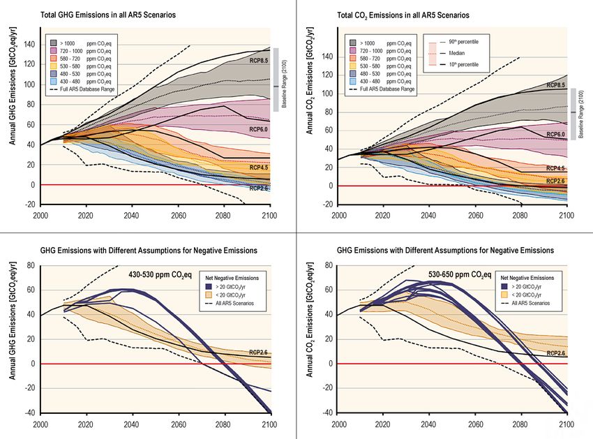
chend weiterverläuft. Diese Szenarien werden sy Die in diesem Synthesebericht betrachteten Szena-
nonym „Business as usual“ (BAU)-Szenarien ge- rien werden Repräsentative Konzentrationspfade
nannt. Hinter Referenz- bzw. Basisszenarien steht (RCP) genannt. Diese RCP beschreiben „vier unter-
die Leitfrage „Was wird sein, wenn nichts geschieht schiedliche Pfade von Treibhausgasemissionen
...?“. Solche Szenarien dienen dem Vergleich (ba- und atmosphärischen Konzentrationen, Luftschad-
seline) zu Szenarien, die alternative Entwicklungs- stoffemissionen und Landnutzung im 21. Jahrhun-
pfade betrachten. dert“ [16]. Sie setzen sich aus einem stringenten
Minderungsszenario (RCP2.6), zwei mittleren Sze-
Policy-Szenarien untersuchen die zukünftigen Aus-
narien (RCP4.5 und 6.0) und einem Szenario mit
wirkungen von Politikentscheidungen. Hinter Policy-
sehr hohen Treibhausgasemissionen (RCP8.5) zu-
Szenarien steht die Leitfrage „Wie wirken sich be-
sammen. Referenzszenarien, die keine zusätzli-
stimmte Politiken aus ...?“.
chen Bemühungen zur Beschränkung von Emissio-
nen beinhalten, entwickeln Pfade, die zwischen
RCP6.0 und RCP8.5 (vgl. Bild 2-3) [16].16
Bild 2-3: Emissionspfade des AR5 im Zeitraum von 2000 bis 2100 für unterschiedliche Szenarien [17]
2.2.2 Einführung zum Emission Gap Report Anstieg der globalen Durchschnittstemperatur auf
(EGR19) deutlich unter 2 °C und auf 1,5 °C begrenzen.
Im Jahr 2019 ist die zehnte Ausgabe des Emission Zudem zeigt der Bericht Wege auf, um diese Emis-
Gap Reports (EGR) der UN erschienen. Der EGR sionslücke zu schließen. Der EGR 2019, welcher
dokumentiert die „Fortschritte bei der Erreichung von einem internationalen Team führender Wissen-
der weltweit vereinbarten Klimaziele“ [8] und ver- schaftler erstellt wurde, betrachtet dabei die neues-
gleicht hierfür die reale Entwicklung der Treibhaus- ten wissenschaftlichen Studien, bspw. die IPCC-
gasemissionen mit den Treibhausgasemissions- Studien. Die Bewertung der Emissionslücke im Jahr
werten, die benötigt werden, um die Treibhausgas- 2030 durch den EGR aus dem Jahr 2018 stützt sich
ziele von 1,5 °C und 2 °C des Pariser Abkommens auf die im Rahmen des Pariser Abkommens im Jahr
[18] einzuhalten. Der ermittelte Unterschied zwi- 2015 vereinbarten National Determined Contributi-
schen dem Status Quo der künftigen Treibhaus on (NDC).
gasemissionen zu den notwendigen Zielwerten,
wird „Emission Gap“ [8] (zu deutsch: Emissionslü- Der EGR 2019 betrachtet zwei Referenzszenarien
cke) genannt. Laut dem EGR 2019 wird diese Emis- sowie NDC-Szenarien und Temperatur-Begren-
sionslücke im Jahr 2030 als die Differenz zwischen zungsszenarien zur Bewertung der Emissionslü-
den projizierten Emissionen unter vollständiger Um- cke. Die beiden Referenzszenarien, das Politiksze-
setzung der national festgelegten Beiträge (NDCs nario 2005 (2005-policies) und das aktuelle Politiks-
[18]) und den Emissionen, die im Pariser Abkom- zenario (Current policy), sind Maßstäbe, mit denen
men (Least Cost Pathways) festgelegt sind, defi- die Fortschritte bei der Emissionsreduzierung ver-
niert. Die Least Cost Pathways stimmen mit den folgt werden können. Das Politikszenario 2005 be-
Zielen des Pariser Abkommens überein, die den trachtet „globale Treibhausgasemissionen, sofern17
ab etwa 2005 keine neue Klimapolitik eingeführt besseren Vergleichbarkeit mit den Werten der Da-
wird“ [8, 17]. tenbank EDGAR wird eine Umrechnung in Gigaton-
nen Kohlenstoffdioxid (CO2) entsprechend den Um-
Dieses Szenario ist das gleiche wie das No Policy- rechnungsvorgaben des AR5-Berichts [7] vorge-
Szenario früherer Berichte. Das No Policy-Szenario nommen.
betrachtet dabei die Entwicklung der globalen Treib-
hausgasemissionen nach dem Jahr 2005, ohne AR5-Szenarien, welche keine zusätzlichen Bemü-
dass weitere Klimaschutzmaßnahmen ergriffen hungen zur Beschränkung von Emissionen (Refe-
werden [19]. renzszenarien) beinhalten, führen zu Entwicklungs-
pfaden zwischen dem Szenario mit mittleren THG-
Das aktuelle Politikszenario betrachtet „Treibhaus- Emissionen (RCP6.0) und dem Szenario mit sehr
gasemissionen, vorausgesetzt, dass alle derzeit hohen THG-Emissionen (RCP8.5). Laut dem Be-
verabschiedeten und umgesetzten Richtlinien (defi- richt der ersten Arbeitsgruppe zum fünften Sach-
niert als legislative Entscheidungen, Ausführungs- standsbericht aus dem Jahr 2013 [20] werden sich
beschlüsse oder gleichwertige Maßnahmen) umge- die zu erwartenden energiebedingten anthropoge-
setzt werden und keine zusätzlichen Maßnahmen nen CO2-Emissionen ohne Landwirtschaft, Forst-
ergriffen werden“ [8]. wirtschaft und sonstige Landnutzung (AFOLU) im
Jahr 2030 zwischen 36,63 Gt CO2 und 50,57 Gt
CO2, im Jahr 2050 zwischen 47,67 Gt CO2 und
2.3 Betrachtung der Zukunft 73,45 Gt CO2, im Jahr 2060 zwischen 54,02 Gt CO2
und 85,51 Gt CO2, im Jahr 2070 zwischen 59,88 Gt
2.3.1 Aussagen im fünften Sachstandsbericht
CO2 und 94,43 Gt CO2 und im Jahr 2100 zwischen
des IPCC
49,98 Gt CO2 und 105,17 Gt CO2 bewegen (vgl. Ta-
Anthropogene CO2-Emissionen belle 2-3) [10].
Im Anhang zum Beitrag der Arbeitsgruppe I „Natur- Laut dem Bericht der ersten Arbeitsgruppe zum
wissenschaftliche Grundlagen“ zum fünften Sach- fünften Sachstandsbericht aus dem Jahr 2013 [20]
standsbericht werden anthropogene Emissionen werden sich die zu erwartenden energiebedingten
aufgelistet. Einen Teil dieser Auflistung stellen die anthropogenen CO2-Emissionen inklusive Land-
anthropogenen CO2-Emissionen, wiederum unter- wirtschaft, Forstwirtschaft und sonstige Landnut-
teilt in anthropogene CO2-Emissionen aus fossilen zung (AFOLU) im Jahr 2030 zwischen 35,09 Gt
Brennstoffen und anderen industrielle Quellen (FF), CO2 und 53,28 Gt CO2, im Jahr 2050 zwischen
anthropogene CO2-Emissionen aus Land- und 45,91 Gt CO2 und 75,58 Gt CO2, im Jahr 2060 zwi-
Forstwirtschaft, Landnutzung (AFOLU) sowie anth- schen 53,03 Gt CO2 und 87,39 Gt CO2, im Jahr
ropogene Gesamt-CO2-Emissionen, dar [10]. Die 2070 zwischen 59,74 Gt CO2 und 95,97 Gt CO2 und
dort vorhandenen Werte sind in Petagramm (1015 g) im Jahr 2100 zwischen 50,68 Gt CO2 und 105,5 Gt
Kohlenstoff pro Jahr (PgC/Jahr) angegeben. Zur CO2 bewegen (vgl. Tabelle 2-4).
Szenario (ohne AFOLU) 2010 2030 2050 2060 2070 2100
RCP6.0
30,77 36,63 47,67 54,02 59,88 49,98
mittlere THG-Emissionen
RCP8.5
32,64 50,57 73,45 85,51 94,43 105,17
sehr hohe THG-Emissionen
Tab. 2-3: Weltweite anthropogene CO2-Emissionen aus fossilen Brennstoffen und anderen industriellen Quellen [Gt CO2] in den
Jahren 2010, 2030, 2050, 2060, 2070 und 2100 (ohne AFOLU); eigene Darstellung und Berechnungen nach [10]
Szenario (inkl. AFOLU) 2010 2030 2050 2060 2070 2100
RCP6.0 34,18 35,09 45,91 53,03 59,74 50,68
RCP8.5 36,60 53,28 75,58 87,39 95,97 105,50
Tab. 2-4: Weltweite anthropogene CO2-Emissionen aus fossilen Brennstoffen und anderen industriellen Quellen [Gt CO2] in den
Jahren 2010, 2030, 2050, 2060, 2070 und 2100 (inkl. AFOLU); Quelle: eigene Darstellung und Berechnung nach [10]18
Landwirtschaft, Forstwirtschaft und andere sultieren, werden mit dem Begriff FOLU (Forstwirt-
Landnutzung (Agriculture, forestry and other schaft und andere Landnutzung) beschrieben [13].
land use, AFOLU)
AFOLU ist für die Ernährungssicherheit und nach- 2.3.2 Aussagen im Emission Gap Report 2019
haltige Entwicklung von großer Bedeutung. Im
AFOLU-Sektor setzen sich die bestimmenden Min- Treibhausgasemissionen [Gt CO2 Äq]
derungsoptionen aus einer Strategie oder mehre-
Laut dem Emission Gap Report des Jahres 2019
ren Strategien zusammen:
werden die gesamten globalen Treibhausgasemis-
• Vermeidung von Emissionen in die Atmosphäre, sionen im Jahr 2030 64 Gt CO2 Äq (in einem 10. bis
indem bestehende Kohlenstoffspeicher in Bö- 90. Perzentilbereich von 60 Gt CO2 Äq bis 68 Gt
den oder der Vegetation erhalten bzw. Emissio- CO2 Äq) betragen, wenn mit einem 2005-policies
nen von Methan und Lachgas verringert werden (no policy)-Basisszenario, also ohne die Einrich-
tung weiterer Klimaschutzmaßnahmen, gerechnet
• Entzug von CO2 aus der Atmosphäre, indem wird.
Kohlendioxid aus der Atmosphäre entzogen und
in bestehenden Kohlenstoffspeichern eingela- In einem Current Policy-Szenario, in welchem die
gert wird (Sequestrierung) derzeitigen getroffenen Vereinbarungen weiterge-
führt werden, werden die Treibhausgasemissionen
• Verringerung der CO2-Emissionen durch Substi- im Jahr 2030 voraussichtlich 60 Gt CO2 Äq (in ei-
tution fossiler Brennstoffe oder von Produkten nem 10. bis 90. Perzentilbereich von 58 Gt CO2 Äq
mit hohem Energieaufwand mittels biologischer bis 64 Gt CO2 Äq) betragen (vgl. Tabelle 2-5 und
Produkte Tabelle 2-6).
Ebenfalls von Bedeutung können Maßnahmen auf
der Nachfrageseite, wie z. B. eine Reduktion von
Abfällen und Verlusten von Nahrungsmitteln oder
eine Veränderung des Ernährungsverhaltens, sein Szenario 2030
[13].
2005-policies (no-policy) 64 (60 – 68)
Die Teilmenge an Treibhausgasemissionen und Current policy 60 (58 – 64)
-entnahmen des AFOLU-Sektors, welche unmittel-
bar aus der vom Menschen erzeugten Landnut- Tab. 2-5: Gesamte globale Treibhausgasemissionen im Jahr
2030 im 2005-policies(no-policy)-Basisszenario und
zung, Landnutzungsänderung und Forstwirtschaft Current Policy-Szenario (Median und 10. bis 90. Per-
(LULUCF) ohne landwirtschaftliche Emissionen re- zentilbereich) in Gt CO2 Äq [8]
Scenario Number Global Estimated temperature Closest cor Emissions Gap in 2030
(rounded to of scena total outcomes responding [GtCO2e]
the nearest rios in set emissions IPCC SR1.5
gigaton) in 2030 50% 66% 90% scenario Below Below Below
[GtCO2e] probability probability probability class 2.0°C 1.8°C 1.5°C in
2100
64
2005-policies 6
(60–68)
60 18 24 35
Current policy 8
(58–64) (17–23) (23–29) (34–39)
Unconditional 56 15 21 32
11
NDCs (54–60) (12–18) (18–24) (29–35)
Conditional 54 12 18 29
12
NDCs (51–56) (9–14) (15–21) (26–31)
Peak: Peak: Peak:
Below 2.0°C 41 1.7-1.8°C 1.9-2.0°C 2.4-2.6°C Higher-2.0°C
29
(66% probability) (39–46) In 2100: In 2100: In 2100: pathways
1.6-1.7°C 1.8-1.9°C 2.3-2.5°C
Tab. 2-6: Globale Treibhausgasemissionen im Jahr 2030 für verschiedene Szenarien (Median und 10. bis 90. Perzentilbereich),
Temperaturauswirkungen und der resultierenden Emissionslücke [8]19
Scenario Number Global Estimated temperature Closest cor Emissions Gap in 2030
(rounded to of scena total outcomes responding [GtCO2e]
the nearest rios in set emissions IPCC SR1.5
gigaton) in 2030 50% 66% 90% scenario Below Below Below
[GtCO2e] probability probability probability class 2.0°C 1.8°C 1.5°C in
2100
Peak: Peak: Peak:
Below 1.8°C 35 1.6-1.7°C 1.7-1.8°C 2.1-2.3°C Lower-2.0°C
43
(66% probability) (31–41) In 2100: In 2100: In 2100: pathways
1.3-1.6°C 1.5-1.7°C 1.9-2.2°C
Below 1.5°C in
Peak: Peak: Peak:
2100 and peak 1.5°C with
25 1.5-1.6°C 1.6-1.7°C 2.0-2.1°C
below 1.7°C 13 no or limited
(22–31) In 2100: In 2100: In 2100:
(both with 66% overshoot
1.2-1.3°C 1.4-1.5°C 1.8-1.9°C
probability)
Tab. 2-6: Fortsetzung
2.4 Übersicht der gesamten Treib Datenbank betrachtet die Emissionen auf den drei
hausgas- und Kohlendioxid- räumlichen Ebenen weltweit, der EU 28 und
emissionen Deutschland. Die anderen beiden Berichte betrach-
ten die Emissionen anhand der in Kapitel 2.2 und
Tabelle 2-7 gibt eine Übersicht zu den gesamten 2.3 vorgestellten Szenarien. Die Daten der CO2 Äq
Treibhausgas- und Kohlendioxidemissionen in Ver- der Jahre 2030, 2050, 2060, 2070 und 2100 des 5.
gangenheit, Gegenwart und Zukunft aus den zu- Sachstandsberichts sind optisch aus Bild 2-3 abge-
vor genannten Quellen [7, 10, 19, 21]. Die EDGAR- lesen.
Fossil CO2 and GHG emissions of 5. Sachstandsbericht des Emissions Gap Report
all world countries – 2019 report zwischenstaatlichen 2019
Ausschusses für Klima
änderungen (IPCC) 2013
Treibhausgas-
emissionen Weltweit EU 28 Deutsch RCP6.0 RCP8.5 2005-policies Current
[Mt CO2] land (no-policy) policy
CO2 15.775,86 4.198,20 1.082,02 / / / /
1970
CO2Äq 24.305,46 5.507,03 1.325,52 / / / /
CO2 15.705,23 4.196,39 1.076,49 / / / /
Vergangenheit
1971
CO2Äq 24.532,22 5.537,72 1.323,49 / / / /
CO2 25.600,66 4.121,66 871,08 / / / /
2000
CO2Äq 35.962,45 5.297,27 1.043,90 / / / /
CO2 33.836,35 3.922,47 816,40 / / 34.176,44 36.896,66
2010
CO2Äq 45.934,04 4.956,27 974,81 / / / /
CO2 36.311,98 3.492,04 786,44 / / / /
2015
CO2Äq 49.113,03 4.499,85 928,69 / / / /
CO2 36.753,96 3.480,15 790,21 / / / /
2016
Gegenwart
CO2Äq / / / / / / /
CO2 37.179,65 3.524,98 787,95 / / / /
2017
CO2Äq / / / / / / /
CO2 37.887,22 3.457,29 752,65 / / / /
2018
CO2Äq / / / / / / /
Tab. 2-7: Treibhausgasemissionen [Mt CO2 Äq] und Kohlendioxidemissionen [Mt CO2] in Vergangenheit, Gegenwart und Zukunft in
Berichten und Szenarien (Stand: 11.12.2019) [7, 10, 19, 21]Sie können auch lesen