URBAN MOBILITY SYMPOSIUM - KARTEN, DATEN, GEOVISUALISIERUNG 11.10.2019 - CITYLAB BERLIN
←
→
Transkription von Seiteninhalten
Wenn Ihr Browser die Seite nicht korrekt rendert, bitte, lesen Sie den Inhalt der Seite unten
URBAN MOBILITY SYMPOSIUM
KARTEN, DATEN, GEOVISUALISIERUNG

11.10.2019 - CITYLAB BERLIN

                                 Organisiert durch:

                 Die Veranstaltung wird finanziell unterstützt durch
             den Regierenden Bürgermeister von Berlin — Senatskanzlei.

         Image: 09-00-1949_06624 Verkeer op Koningssluis by IISG on Flickr
URBAN MOBILITY SYMPOSIUM
Proceedings

INHALT
Visualisierung des Bewegungsverhaltens mit einer erweiterten Flowstrates Darstellung p.4
anhand der Modellregion Hochfranken
Christoph Menzel
hin&weg - Analysis and Visualisation Tools for the Study of Urban 				 p.8
and Regional Migration Data
Maria Turchenko
Scalability of OD-data visualizations								p.12
Ilya Boyandin
Transport advocacy through smart data analysis and visualisation				                 p.15
William Jones & Santosh Seshadri
Mobility as a Service – eine Chance für Menschen in Armut? 					                     p.19
GIS-basierte Untersuchung vierer Ridepooling-Angebote in Hamburg
Christoph Aberle
Urban Transects and Trunk Roads - Observations in Hamburg					                       p.24
Timotheus Klein & Sebastian Clausen
Personal exposure to environmental stressors while commuting: 					           p.28
Exploring on-site experiences using Walking Interviews and qualitative GIS
Heike Marquart & Uwe Schlink
More LA: Transforming Parking to Places in Los Angeles						                         p.32
Fabio Galicia, Lucy Helme, Dave Towey, Christian Derix

3

PROGRAMMAUSSCHUSS
VORSITZ

     Sebastian Meier, Technologiestiftung Berlin
     Johannes Kröger, HafenCity University, Hamburg

MITGLIEDER

     Sigrun Beige, Telefónica NEXT — Location & Mobility Analytics
     Marian Dörk, Fachhochschule Potsdam
     Julia Gonschorek, EASC eV.
     Anita Graser, Austrian Institute of Technology, Wien
     Katharina Jacob, Fachhochschule Potsdam
     Alexandra Kapp, Technologiestiftung Berlin
     Felix Kunde, Zalando
     Nicolas Neubauer, HERE, Berlin
     Charlotte Pusch, Technische Universität Hamburg
     Raphael Reimann, Moovel
     Jochen Schiewe, HafenCity University, Hamburg
     Harald Schernthanner, Universität Potsdam
     Lucia Tyrallova, Universität Potsdam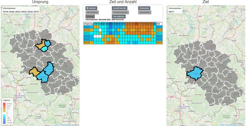
URBAN MOBILITY SYMPOSIUM
Proceedings

Abbildung 2. Betrachten einer Region auf der linken Karte.

Christoph Menzel (christoph.menzel.2@gmail.com)
Hochschule für Angewandte Wissenschaften Hof

VISUALISIERUNG DES BEWEGUNGS-
VERHALTENS MIT EINER ERWEITER-
TEN FLOWSTRATES DARSTELLUNG
ANHAND DER MODELLREGION HOCH-
FRANKEN
Keywords: Visual Analytics, Bewegungsdaten, Flowstrates      Paper beantwortet werden:

1. EINLEITUNG                                                •   Wie kann der zeitliche Verlauf von Bewegungen ver-
Dieses Paper befasst sich mit der visuellen Unterstützung        anschaulicht werden?
der Analyse des Bewegungsverhaltens in der Modellre-         •   Wie lässt sich ein Verhältnis zwischen aus- und
gion Hochfranken. Dazu sind die Veränderungen des                eingehenden Bewegungen darstellen, wenn mehrere
Bewegungsverhaltens im Verlauf eines Tages zwischen              Regionen gegenübergestellt werden?
Regionen relevant sowie Unterschiede zwischen Bewe-          •   Wie kann ein Vergleich zwischen zwei Datensätzen
gungsdaten aus zwei verschiedenen Zeiträumen oder                visualisiert werden?
Quellen. Die Visualisierung des Bewegungsverhaltens ist
ein wichtiges Hilfsmittel der Analyse. Aus den genannten     Für die aufgeführten Fragestellungen werden in Kapitel 2
Kriterien für die Analyse lassen sich folgende Fragestel-    vorhandene Visualisierungen auf deren Eignung geprüft.
lungen für die Visualisierung ableiten, die in diesem        Die ausgewählte Darstellung wird in Kapitel 3 beschrieben
5

und es werden hinzugefügte Funktionalitäten aufgezeigt,       3.2 Aufbau der Darstellung
die für die Beantwortung der aufgeführten Fragestel-          Flowstrates weist eine vertikal dreigeteilte Ansicht auf.
lungen erforderlich sind. In Kapitel 4 wird anhand einer      Auf der linken und rechten Seite befindet sich je eine
Fallstudie auf Basis der Region Hochfranken exemplar-         Karte. Die linke Karte ist für ausgehende, die rechte Karte
isch aufgezeigt, wie die Visualisierung zur Analyse des       für eingehende Bewegungen zuständig. Zwischen beiden
Bewegungsverhaltens genutzt werden kann. Abschließend         Karten befindet sich eine Tabelle, deren Zeilen die Bewe-
werden die Ergebnisse zusammengefasst und ein Ausblick        gungen von einer Ursprungs- in eine Zielregion repräsen-
auf zukünftige Erweiterungen gegeben.                         tieren. Durch die Spalten der Tabelle erfolgt eine Untertei-
                                                              lung in Zeitintervalle. Jede dabei entstehende Zelle stellt
2. STAND DER WISSENSCHAFT                                     eine zeitabhängige Bewegung dar. Je nach deren Stärke
Die Herausforderung bei der Visualisierung von Bewe-          wird eine farbliche Unterscheidung vorgenommen. Das
gungen besteht darin, räumliche und zeitliche Infor-          Betrachten einer zeitabhängigen Bewegung in der Tabelle
mationen verständlich und übersichtlich abzubilden. Es        hat zur Folge, dass die beiden beteiligten Regionen der
existieren statische Darstellungen wie Flow Maps (Tobler,     Bewegung auf der jeweiligen Karte anhand der Stärke
1987) oder Edge Bundling (Holten et al., 2009), die keine     der zeitabhängigen Bewegung eingefärbt werden, wie in
zeitlichen Aspekte aufweisen. Mit animierten Darstellun-      Abbildung 1 dargestellt. Durch das Auswählen einer oder
gen kann der zeitliche Verlauf aufgezeigt werden (Becker      mehrerer Regionen auf den Karten ist es möglich, die
et al., 1995). Bei vielen Bewegungen und Regionen ist dies    Tabelle auf die jeweiligen Bewegungen zu beschränken.
unübersichtlich und schwer nachverfolgbar. In einem in-       Bei jeder Auswahl des Anwenders wird die Tabelle erneut
teraktiven Ansatz wie MobilityGraphs (von Landesberger        aufgebaut, wodurch die Farbwerte im Kontext der aktuel-
et al., 2016) mit separaten Darstellungen für die zeitliche   len Auswahl neu berechnet werden.
und räumliche Komponente sind alle Informationen
vorhanden. Dieser erfordert jedoch tiefere Einarbeitung
durch den Anwender. Mit Flowstrates (Boyandin et al.,
2011) existiert eine interaktive Darstellung, um Bewegun-
gen anhand zeitlicher und räumlicher Kriterien übersicht-
lich und detailliert darzustellen.

3. FLOWSTRATES

3.1 Definitionen
Bevor die Anwendung im Detail betrachtet werden kann,
                                                              Abbildung 1. Ursprüngliche Flowstrates Visualisierung, in welcher die
ist die Definition folgender Begriffe erforderlich:           Ursprungsregion (links) und Zielregion (rechts) anhand der Stärke
• Bewegung: Ortsveränderung von Personen zwischen             der betrachteten zeitabhängigen Bewegung eingefärbt werden. In der
                                                              Tabelle (Mitte) befinden sich die Bewegungen untereinander, vertikal
     zwei unterschiedlichen Regionen.                         zeitlich unterteilt. (Boyandin et al., 2011)
• Zeitabhängige Bewegung: In einem bestimmten
     Zeitintervall startende Bewegung.                        3.3 Verbesserungen des ursprünglichen Ansatzes
• Bewegungsverhalten: Alle in einem Datensatz vor-            Mit dem ursprünglichen Ansatz kann geklärt werden, ob
     kommenden Bewegungen.                                    und wie sich die Bewegungsstärke im zeitlichen Verlauf
• Stärke einer Bewegung: Anzahl der sich bewegenden           verändert. Mit veränderten Funktionalitäten kann dies
     Personen.                                                detaillierter beantwortet werden. Um Datensätze mitein-
• Auswählen: Temporäres Einschränken der Ursprungs-           ander zu vergleichen oder das Verhältnis zwischen aus-
     und/oder Zielregionen durch den Anwender.                und eingehenden Bewegungen zu bestimmen, müssen
• Betrachten: Untersuchen einer Region, eines Zeitin-         neue Funktionalitäten ergänzt werden.
     tervalls oder einer Bewegung. Die tatsächliche Aus-
     wahl bleibt unverändert.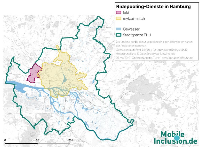
URBAN MOBILITY SYMPOSIUM
Proceedings
3.3.1 Gesamtstärke der Bewegungen
Im ursprünglichen Ansatz besteht keine Möglichkeit, die
Stärke von Bewegungen, unabhängig des Zeitintervalls,
anzuzeigen. Dies wurde ergänzt, da sich daran in einem
ersten Schritt erkennen lässt, welche Regionen über den
gesamten Zeitraum am häufigsten als Ursprung oder Ziel
dienen.
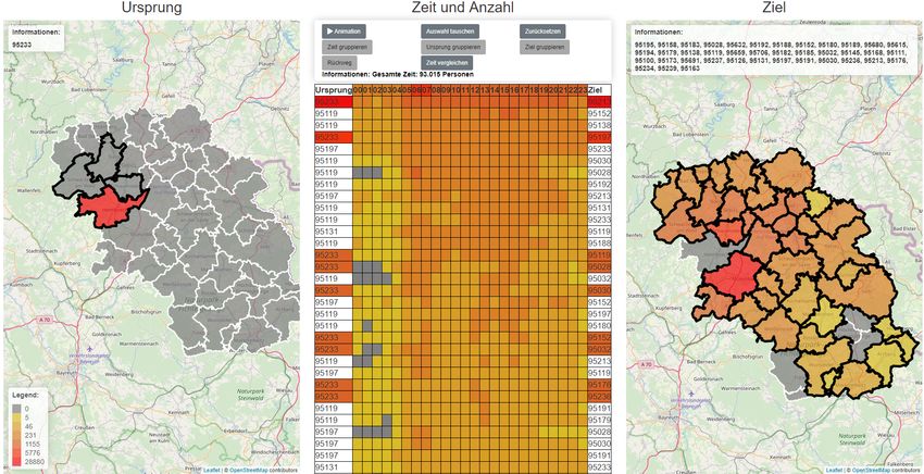
3.3.2 Betrachten einer Region
Beim Betrachten einer Region auf der Karte werden die Abbildung 3. Vergleich zwischen Hinweg und Rückweg ausgewählter Be-
wegungen über den gesamten Zeitraum. Ist die Stärke der ausgehenden
beteiligten Zeilen der Tabelle farblich anhand der Bewe- Bewegung größer als die der eingehenden, wird dies in Orangetönen
gungsstärke während des gesamten Zeitraums markiert. dargestellt, andernfalls in Blautönen.
Außerdem werden alle betroffenen Regionen auf der
entgegengesetzten Karte in denselben Farben eingefärbt. 3.3.5 Vergleich zweier Datensätze
In der Kartenansicht der betrachteten Region wird diese Um Unterschiede im Bewegungsverhalten zwischen zwei
farblich anhand der Gesamtstärke aller betroffenen Bewe- Datensätzen aufzuzeigen, wird die Anwendung um eine
gungen gekennzeichnet, was in Abbildung 2 zu erkennen Vergleichsfunktionalität ergänzt. Voraussetzung dafür
ist. Die drei weiteren schwarz umrahmten Regionen auf ist, dass beide Datensätze ein einheitliches Datenschema
der linken Karte sind hervorgehoben, weil diese Teil der nutzen, was verwendete Zonierung und Zeitintervalle
vom Anwender getroffenen Auswahl sind. Bei weiß um- betrifft. Differenzen in der Bewegungsstärke zwischen
rahmten Regionen auf der rechten Karte existieren keine beiden Datensätzen werden farblich dargestellt. Erhöht
Bewegungen aus der Ursprungsregion. Des Weiteren sich die Bewegungsstärke werden Orangetöne verwendet,
besteht die Option, ein Zeitintervall festzulegen. Beim verringert sich die Bewegungsstärke Blautöne.
Betrachten einer Region erfolgt dann die Färbung der Re-
gionen in beiden Karten ausschließlich anhand der Stärke 4. Auswertung der Ergebnisse anhand der Fallstudie
der zeitabhängigen Bewegungen. Hochfranken
3.3.3 Animation 4.1 Datenbasis
Obwohl in Kapitel 2 aufgeführt wird, dass Animationen Die Arbeiten dieses Papers sind im Rahmen des For-
als alleinige Visualisierung ungeeignet sein können, lässt schungsprojektes Mobilität Digital Hochfranken
sich Flowstrates um eine solche Option erweitern. Es entstanden, in welchem das Bewegungsverhalten in der
wird eine Einfärbung der Regionen anhand der Stärke der Modellregion Hochfranken analysiert wird. Als Daten-
Bewegungen im jeweiligen Zeitintervall vorgenommen. basis dienen Bewegungsdaten von Mobiltelefonen eines
Die Animation der Bewegungen berücksichtigt die vom Telekommunikationsunternehmens, welche aus einem
Anwender getroffene Auswahl. Da der Anwender einzelne Analysezeitraum vom 01. bis 29. März 2017 stammen.
Bewegungsinformationen interaktiv untersuchen kann, Es sind ausschließlich stündliche Bewegungen für die
dient die Animation als unterstützende Komponente. Wochentage Montag bis Donnerstag aufgeführt. Die
Bewegungen wurden auf Ebene der Postleitzahlengebiete
3.3.4 Rückweg erfasst. Bewegungen, die nur eines der beiden Gebiete als
Mit entgegengesetzten Bewegungen lassen sich Regionen Ursprungs- bzw. Zielregion aufweisen, sind ebenso wie
in ein Verhältnis stellen. Für jedes Zeitintervall wird an- Durchgangsverkehr nicht enthalten. Mit Erkenntnissen
hand der ausgewählten Regionen die Differenz zwischen aus dem Projekt sollen Simulationen erstellt werden, bei
aus- und eingehenden Bewegungen berechnet. Ist die denen das tatsächliche Bewegungsverhalten nachempfun-
berechnete Bewegungsstärke negativ erfolgt das Einfär- den wird.
ben in Komplementärfarben, siehe Abbildung 3.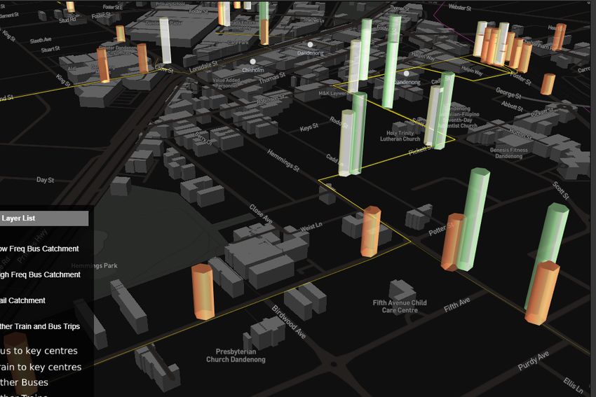
7

4.2 Veränderung der Bewegungsstärke                           einen zeitlichen Verlauf zu analysieren. Die anfangs
Mit der Darstellung kann festgestellt werden, dass sich die   aufgeführten Fragestellungen lassen sich mit den ergänz-
Bewegungsstärke im Verlauf eines Tages deutlich ändert.       ten Funktionalitäten beantworten. Das Betrachten einer
Besonders morgens und zwischen Mittag und Nachmittag          Region auf der Karte ermöglicht es, die zugehörigen
sind gesamtheitlich die meisten Bewegungen vorzufin-          Zielregionen auf der entgegengesetzten Karte anhand der
den. Die in Abbildung 2 getroffene Auswahl deutet diese       entsprechenden Bewegungsstärke hervorzuheben. Durch
Verhaltensweise an. Da die Daten für Wochentage ermit-        das Animieren der Bewegungen werden Veränderungen
telt wurden, könnte dies auf Bewegungen zu Schulen oder       der Bewegungsstärke im zeitlichen Verlauf zusätzlich
Arbeitsplätzen zurückzuführen sein. Vormittags, abends        herausgestellt. Mit der Rückwegsansicht können Regionen
und nachts finden vergleichsweise weniger Bewegungen          in Relation zueinander gestellt werden. Damit wird
statt. Außerdem weisen städtische Gebiete mehr Bewe-          das Verhältnis von aus- und eingehenden Bewegungen
gungen auf als ländliche. Die hinzugefügten Funktion-         deutlich, wodurch sich Rückschlüsse auf die Infrastruktur
alitäten aus Abschnitt 3.3.1 bis 3.3.3 unterstützen den       einer Region ziehen lassen. Es ist möglich, Datensätze zu
Anwender bei der Analyse des Bewegungsverhaltens.             vergleichen, wodurch starke Abweichungen in komple-
                                                              mentären Farben ersichtlich werden. Dies kann bei der
4.3 Rückweg                                                   Analyse des Bewegungsverhaltens zu unterschiedlichen
Die beschriebene Ansicht des Rückweges gibt das Verhält-      Zeiträumen, aus verschiedenen Datenquellen oder zum
nis aus- und eingehender Bewegungen zwischen Regionen         Vergleich mit Simulationsergebnissen genutzt werden.
an. In Abbildung 3 ist erkennbar, dass sich die oberen        Erkenntnisse, die aus der Darstellung hervorgehen,
drei Bewegungen im zeitlichen Verlauf deutlich von            lassen sich beispielsweise für den öffentlichen Personen-
den unteren drei unterscheiden. Die oberen drei zeigen        nahverkehr nutzen, um zu verifizieren, ob sich deren
Bewegungen zwischen Münchberg und den drei Postle-            Routen mit häufig aufgesuchten Bewegungen decken bzw.
itzahlengebieten der Stadt Hof, die unteren drei zwischen     ob angebotene Abfahrtszeiten während Intervallen mit
Münchberg und periphereren Regionen. Morgens finden           hoher Bewegungsstärke stattfinden. Weiterführend wäre
von Münchberg in die Stadt Hof mehr Bewegungen statt          eine offene Frage, wie eine dynamische Zonierung der
als entgegengesetzt. Ab Mittag kehrt sich dieses Verhält-     Regionen erreicht werden kann, um fein- und grobgranu-
nis um. Bei den anderen drei Bewegungen zeichnet sich         larere Analysen durchzuführen.
ein gegensätzliches Bild ab. Das vermehrte Aufkommen
von Schulen und Arbeitsplätzen in Hof im Vergleich zu         6. Referenzen
                                                              Becker, R. A., Eick, S. G., & Wilks, A. R. (1995). Visualizing network data.
Münchberg, aber wiederum im Vergleich von Münchberg           IEEE Transactions on Visualization and Computer Graphics, 1(1), 16–28.
zu den peripheren Regionen, könnte eine Ursache dessen        Boyandin, I., Bertini, E., Bak, P., & Lalanne, D. (2011). Flowstrates: An
sein.                                                         Approach for Visual Exploration of Temporal Origin-Destination Data.
                                                              Computer Graphics Forum, 30(3), 971–980.
                                                              Holten, D., & van Wijk, J. J. (2009). Force-Directed Edge Bundling for
4.4 Vergleich zweier Datensätze                               Graph Visualization. Computer Graphics Forum, 28(3), 983–990.
Der Vergleich zweier Datensätze soll im Projekt dafür         von Landesberger, T., Brodkorb, F., Roskosch, P., Andrienko, N., Andrien-
genutzt werden, das Bewegungsverhalten beispielsweise         ko, G., & Kerren, A. (2016). MobilityGraphs: Visual Analysis of Mass
                                                              Mobility Dynamics via Spatio-Temporal Graphs and Clustering. IEEE
zu unterschiedlichen Jahreszeiten oder im Vergleich           Transactions on Visualization and Computer Graphics, 22(1), 11–20.
zwischen Wochentagen und Wochenende zu analysieren.           Tobler, W. R. (1987). Experiments In Migration Mapping By Computer.
Die im Rahmen des Projektes erstellten Simulationen           The American Cartographer, 14(2), 155–163.

können mit den tatsächlichen Bewegungen verglichen            [33] World Air Map by Plume Labs. Available: https://air.plumelabs.com/
                                                              en/. [Accessed 23-Aug-2019]
werden. Mit der Darstellung besteht die Möglichkeit, die
                                                              [34] N. Yau, “Visualizing Incomplete and Missing Data”, FlowingData, 30-
Ergebnisse der Simulation zu verifizieren, da stark abwe-     Jan-2018. Available: https://flowingdata.com/2018/01/30/visualizing-in-
ichende Ergebnisse deutlich auffallen.                        complete-and-missing-data/. [Accessed: 20-Jun-2019]
                                                              [35] Yellow Dust. Available: http://yellowdust.intheair.es/. [Accessed 21-
                                                              Jun-2019]
5. Fazit
Durch die dreigeteilte Darstellung besteht eine anschauli-
che und strukturierte Übersicht, um Bewegungen über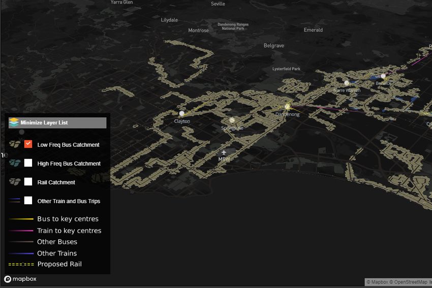
URBAN MOBILITY SYMPOSIUM
Proceedings

Figure 4. Chord and sankey diagrams in the alpha version of hin&weg software.

Maria Turchenko (m_turchenko@ifl-leipzig.de) & Francis Harvey (f_harvey@ifl-leipzig.de)
Leibniz Institute for Regional Geography

HIN&WEG —
ANALYSIS AND VISUALISATION TOOLS
FOR THE STUDY OF URBAN AND
REGIONAL MIGRATION DATA

Keywords: analysis tools, visualisation tools, statistical                      demographic changes and their impacts, e.g., changing
migration data, origin-destination, participatory design                        demands of the transportation networks (Andrienko et
                                                                                al., 2017). While technologically the challenges in this
1. INTRODUCTION                                                                 application are (at the moment) not ground-breaking nor
The digitalisation of public administrations opens up                           cutting edge developments, the application address the
many intriguing possibilities for improving the use of                          almost complete absence of any software to support time/
demographic data. The complexity of this data means                             space analysis integrated with visualisation of official
visualisation tools are frequently required and ideally                         demographic data. Following a participative design ap-
coupled with analysis functionality to support analysis.                        proach that aims to assure the basic suite of analysis and
In the hin&weg project we are developing an innovative                          visualisation tools is useful for administrative staff, the
and integrated analysis and visualisation application (also                     data architecture we develop in the first phase can support
called hin&weg) for administrative work with urban and                          further extensions and technological developments that
suburban migration information from official registry                           support new modes of use among staff, and ideally, the
data. The analysis and visualisation of the administrative                      general public. Due to the protected nature of official
statistical records on migration, inner-city movements                          registry data, the software we develop currently can be
and commuting can help reveal changes and help develop                          deployed also on individual and isolated computers, e.g.,
valuable insights into transformations and the process-                         in a statistical office. Often municipalities lack the tools
es, such as of neighbourhood gentrification and up- and                         to visualise and analyse such complex data. This suggests
downgrading. This tool is also helpful for understanding                        that having an application like hin&weg alone will be
9

innovative for most cities. We describe in this paper and       facilitate the visualisation of diverse urban and regional
presentation the software architecture and preliminary          registry data to help with analysis and development of
functionality, which we will developing in the coming 18        policy. It uses a very different software architecture and
months with cities participating in the hin&weg project.        implementation.

2. BACKGROUND                                                   3. CURRENT HIN&WEG SOFTWARE ARCHITECTURE
The project hin&weg in Leibniz Institute for Regional           The software development follows the principles of
Geography (IfL) involves the development of tools for the       modularity and uses node.js modules (nodejs.org) and
analysis and visualisation of this administrative data. It is   JavaScript libraries. It is built with the Electron framework
an ongoing research project (2019-2021). It will produce        (electronjs.org). The development follows a model-view
in a cross-platform software package. The development           controller pattern, which facilitates the separation of data
cooperates with participants from ten German cities, the        handling from data representation. This pattern allows
German Institute of Urban Affairs (Difu) in Berlin and          us to produce several different front-end outputs from
software development company Delphi IMM from Pots-              the OLAP data cube (npmjs, 2018). The software includes
dam.                                                            models of geodata, table attributive data, a combiner and
Visualisations help city statisticians, city planners and       a time-related aggregation model. Data representations
other expert municipal actors identify patterns and flows       are provided through several views (map, table, line graph,
to support decision-making processes (Ding et al., 2018).       diagrams and database), described in detail later.
Such visualisations can also reach political decision mak-      The generic space/time representation of the hin&weg
ers and the interested public to help them gain insight         data follows the geo-relational model (De Paoli and
into recent and even ongoing processes. Coupling analysis       Miscione, 2011; Chrisman, 2006) extended through the
with visualisations has been very successful (Rudwick,          data cube to support time series analysis. Following this
1976; Ware, 2008; Börner, 2015; Tversky, 2019)                  model, hin&weg data consists of geographic data linked to
Precursors of the current hin&weg project can be traced         attribute data based on the shared id of the administrative
back to 2004. It went through several versions with differ-     areas. The current import format for the geodata is shape-
ent architectures and functionalities, but all of them were     file (geojson remains a possibility) and the attributive data
built around the concept of data visualisation combined         must be provided as a csv-file with header information
with analytical functionality (figure 1). The data was added    for future meta-data fields (e.g., attribute names, time
manually by the professional staff at IFL and users were        periods, etc).
not able to perform import by themselves.

                                                                Figure 2. Simplified overview of hin&weg data processing.

                                                                 To provide not only a visual representation of the data,
                                                                but to support its exploration and knowledge discovery
                                                                interactive visualisations are combined with an analytical
                                                                functionality in the hin&weg interface (figure 3). It is built
                                                                with d3.js in combination with react.js and ramda.js.
Figure 1. A previous version of the hin&weg from 2017.
                                                                4. PROJECT DEVELOPMENT CYCLE
 The current version, under development, integrates analy-      The project development cycle for this version of hin&weg
sis and visualisation tools from the previous versions. They    commences in August 2018 and will last three years. It
should be simple enough for elementary uses and help            includes three stages of software development: alpha, beta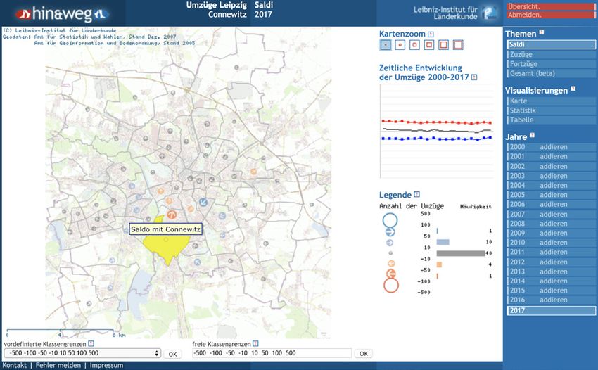
URBAN MOBILITY SYMPOSIUM
Proceedings

and release versions. Each version will be developed in a      data for the chosen years will be aggregated for each ad-
one-year period.                                               ministrative unit.
                                                               There are three diagram types built-in the Alpha-Version.
                                                               These are bar chart, sankey diagram and chord diagram
                                                               (figure 4). The diagrams have mouseover information
                                                               windows and can be filtered with a slider showing only the
                                                               highest values of the flows. The table view represents data
                                                               in form of table with three columns: origin, destination
                                                               and value. The data here can be re-ordered and filtered.
                                                               All the diagrams and table are responsive for the user’s
                                                               selection of administrative area, representation mode and
                                                               years.
                                                               A line graph covers the whole time period of the import-
                                                               ed data and has mouseover functionality, showing exact
Figure 3. hin&weg alpha version interface.                     values for incoming, outgoing flows and their difference.
                                                               Database view include basic SQL-query functionality.
The focus of the Alpha-Version is the development of the       The Beta-Version will focus on improving import process,
stable data import and its storage and retrieval. Currently    developing export functionality and additional visuali-
the Alpha-Version is with participating cities for testing.    sations and analytical functions. Also, the future devel-
At this point we can only provide more details about the       opment includes creating a windowing system for user
Alpha-Version and our first ideas for the Beta-Version.        interface allowing users to decide how many different
During the Alpha-Version development we resolved some          visualisations they want to have at the screen at the same
important challenges for data import. Administrative           time and realign them. The second cycle of development
registry data comes in the form either of lists or matrices    begins after a workshop with the participating cities in
with numerical values for demographic characteristics          November 2019 to prioritise and fine-tune functionality.
according to origin/destination or cumulative values. It       These developments are at first glance technologically
can include several attributes, such as gender, age, marital   modest, but have vast innovative potential in city/commu-
status, etc. Some matrices indicate calculations of changes    nal administrations. In this context, data protection and
between specific data collection time points. Others record    its implementation are important to mention. Reflecting
just the observations and the calculations remain to be        the high emphasis placed in city administrations on data
done. Both involve different data-handling, even though        security, hin&weg is a stand-alone software with an in-
the analysis and visualisations are in the end identical.      ternalised data store that does not require an internet con-
These involve issues to resolve as well in the future.         nection. The software is available for Mac, PC and Linux
The import function is designed to be easy and under-          (Ubuntu) operating systems.
standable for the administrative workers. Thus, the system
will alert error messages with explanations if ids are not     5.PARTICIPATORY DEVELOPMENT OF HIN&WEG
identical in both data sources, or if the formatting of the    The meaningful representation of this data to politi-
data does not correspond to the established format. It is      cians or public is a way to support the productive dialog
possible to upload more than one tabular data file, each       between all participating parties (Boyandin et al., 2011;
representing one year time interval. Map view represents       Contreras-Ochando et al., 2018). This theory has been
data as choropleth map visualisation of the incoming and       demonstrated many times by academics (Jankowski
outgoing flows. The current Alpha-Version only supports        and Nyerges, 2003). It is the innovative emphasis of the
an equal intervals classification. For analysis, the user      hin&weg software. Because of city/communal control of
chooses the administrative area by clicking on the map or      data and stringent legal requirements, the project stakes
from the dropdown list. He should also choose the repre-       out no specific public access ambitions beyond developing
sentation mode: outgoing/incoming flow or differences.         a publicly available version of hin&weg. The specifics of
Additionally, he should choose the years for analysis. The     the public version will be discussed and determined in
11
the coming two years with the project advisory board. The and innovative city planning.
cities and communes have completely flexibility in this The final product of the project is a multi-purpose hin&-
regard. The software could be provided online, installed on weg application. This presentation describes the principles
public kiosks, etc. Data access can also be handled flexibly. and the concepts behind the development of the hin&weg
Currently, we need to strive to develop needed function- analysis and visualisation tools and explains the partic-
ality for the cities and communes. It is important to take ipatory process. By helping create a useful analysis and
a piece of humble pie and recognise we know little how visualisation tool, we believe hin&weg will contribute to
cities carry out the analytical and related visual work re- the digitalisation of German city administration and open
quired and desired using information technology. Hence, up new possibilities for participation. We look forward to
the participatory process emphasises the involvement of sharing more information about hin&weg in the coming
practitioners who determine how to best support planning years.
processes, consider which visualisation types and types of
user interactions are preferable (Spinuzzi, 2005; Sand- 7. REFERENCES
Andrienko, G., Andrienko, N., Chen, W., Maciejewski, R., & Zhao, Y.
ers & Brandt, 2010). For example, we face questions that (2017). Visual analytics of mobility and transportation: State of the art
include: do city staff tend to analyse the data in tables, and further research directions. IEEE Transactions on Intelligent Trans-
portation Systems, 18(8), 2232-2249.
visualisations, work with both, or develop feedback loops
Börner, K. (2015). Atlas of knowledge : anyone can map. Cambridge,
among analysis processes and visualisation processes? Or, Massachusetts: The MIT Press.
is there no clear and dominant approach, but the actual Boyandin, I., Bertini, E., Bak, P., & Lalanne, D. (2011, June). Flowstrates:
choice is dominated by other parameters (experience, An approach for visual exploration of temporal origin‐destination data.
In Computer Graphics Forum (Vol. 30, No. 3, pp. 971-980). Oxford, UK:
work culture, IT-skills, etc)? How much variation do we Blackwell Publishing Ltd.
find? The participation of city administration staff will Chrisman, N. R. (2006). Charting the unknown. Esri Press.
shed light on this in the coming months. Contreras-Ochando, L., Font-Julián, C. I., Nieves, D., & Martínez-
The common method of a participatory design is a whole Plumed, F. (2018). How Data Science helps to build Smart Cities: Valencia
as a use case. In Conference on Small and Medium Smart Cities (pp.
day workshops with the stakeholders and other interested 14-15).
parties of the future software. The first hin&weg work- De Paoli, S., & Miscione, G. (2011). Relationality in geoIT software
shop took place in March 2019 as a focus group discussion development: How data structures and organization perform together.
Computers, Environment and Urban Systems, 35(2), 173-182.
and was focused on defining data formats, basic pref-
Ding, L., Meng, L., Yang, J., & Krisp, J. M. (2018). Interactive visual explo-
erable visualisation types and analytical functions. The ration and analysis of origin-destination data. Proceedings of the ICA.
next ‘user-workshop’ for Alpha-Version users will held Jankowski, P., & Nyerges, T. (2003). GIS for group decision making. Boca
Raton, FL: CRC Press.
in November 2019. In the following 18 months we will be
using established usability testing formats including focus Kuniavsky, M. (2003). Observing the user experience: a practitioner’s
guide to user research. Elsevier.
groups, in-situ software walk-throughs, A/B questions,
Rudwick, M. J. (1976). The emergence of a visual language for geological
questionnaires and telephone interviews. Usage of several science 1760—1840. History of science, 14(3), 149-195.
different methods has been proven to provide a better Sanders, E. B. N., Brandt, E., & Binder, T. (2010, November). A frame-
work for organizing the tools and techniques of participatory design.
overview and more insights. (Kuniavsky, 2003).
In Proceedings of the 11th biennial participatory design conference (pp.
The final version of the software will be distributed at the 195-198). ACM.
concluding workshop in mid-2021. Software and data Spinuzzi, C. (2005). The methodology of participatory design. Technical
communication, 52(2), 163-174.
license arrangements, or their absence (open), will be de-
Tversky, B. (2019). What Makes a Map Good. Medium Retrieved
termined in the project advisory group by this point. 22Jul2019, 2019, from https://modus.medium.com/what-makes-a-map-
good-4db0de3b2cec.
6. RESULTS AND OUTLOOK Ware, C. (2008). Visual thinking for design. New York City: Morgen
Kaufmann.
At this stage in the project, this paper and corresponding
npmjs. 2018. cubus. [ONLINE] Available at: https://www.npmjs.com/
presentation provide basic information about software package/cubus. [Accessed 4 September 2019].
aspects of the ongoing hin&weg project. The participato- electronjs. Electron. [ONLINE] Available at: https://electronjs.org/. [Ac-
ry approach emphasises the innovative potential of this cessed 4 September 2019].
software to support analysis and formulation of policy in nodejs. Node.js. [ONLINE] Available at: https://nodejs.org/en/. [Accessed
4 September 2019].
completely new ways, which can help guide a more liveableURBAN MOBILITY SYMPOSIUM
Proceedings
Figure 3. Flowmap.query, an exploratory visualization tool for the analysis of OD-data with attributes backed by an efficient database.
Ilya Boyandin (ilya@boyandin.me)
Teralytics
SCALABILITY OF OD-DATA
VISUALIZATIONS
Keywords: geographic data visualization, movement of to create interactive geographic flow maps from datasets
people, mobility, transportation, flow maps, scalability uploaded to Google spreadsheets. Since it was published
few months ago, hundreds of datasets from all around the
1. INTRODUCTION world have been visualized with it.
Understanding mobility patterns is important for This simple tool, however, only works well for relative-
fields like migration studies, urban and transportation ly small datasets (tens of thousands rows). The size of
planning, epidemiology, ecology, and disaster response. OD-data depends quadratically on the number of loca-
Origin-destination data (OD-data) are often used in this tions involved. It can quickly grow to hundreds of millions
context for analysing numbers of movements between of rows when flow attributes like time, mode of transport,
geographic locations. We believe that many OD-datasets duration are added to the dataset. Such large datasets
remain under-analysed. The reason for that is that not cannot be entirely visualized in one image. Their analysis
many analysis tools are available today that are designed requires the use of summarization and interactive explo-
specifically for this kind of data and that are, at the same ration techniques. Moreover, ensuring smooth interac-
time, easy to use. tivity and short query response times necessary for such
To improve this situation we published and open-sourced interactive analysis requires using an efficient database
Flowmap.blue1, an online tool which makes it very easy for executing the queries.13
At the company Teralytics we are building exploratory To address these two problems we implemented an
tools for the analysis of aggregated data on movement of adaptive clustering approach. Locations within a certain
people in cities and countries with the purpose of improv- distance from each other (the distance depends on the
ing transportation and mobility services. Scalability to current map zoom level) are clustered together (Figure 1b,
the growing data sizes is an important challenge we are d). The clusters are positioned in the centers of mass-
facing. In this article we discuss some of the technological es of the locations constituting them (the locations are
solutions we have been working on to address this chal- weighted by their total in-/out flows). After the location
lenge and the tools we have published and open-sourced to clusters are formed, flows are aggregated by summing up
make these solutions available to the broad public. the magnitudes of the flows connecting the constituents
of the clusters.
We are using a simple and very efficient density-based
clustering algorithm implemented in the Supercluster2 li-
brary. Instead of the automated clustering approach, tak-
ing an existing administrative area hierarchy may result
in more meaningful and familiar clusters. However, with
the former it is possible to produce a separate clustering
for each map zoom level providing for a smoother user
experience. In any case, the flow aggregation step doesn’t
depend on any particular algorithm and can be applied to
any clustering.
The clustering level adapts to the map zoom making sure
that not too many flows need to be drawn and that all the
drawn flows are not too short. Flow lines which are too
short are summarized as cluster-internal flows and are
Figure 1. Bus rides in São Paulo. a) The original “messy” version with too represented as part of the location totals by the circles of
many overlapping locations and flows. b) A clustered version of the same
dataset showing high-level patterns. Relocations in Australia c) The orig-
varying sizes. When zooming in, the clusters will gradual-
inal version with the most important flows being too short to be visible. ly expand, so the level of summarization will automatically
d) Clustered version making high-level patterns visible. The circle sizes
show the locations’ in-/out totals and include internal flows. adapt to the map viewport.
This approach makes it possible to visualize and explore
2. SCALABILITY OF FLOW MAPS very large OD-datasets providing a useful summary at
In our tools we use flow maps as the main geographic first and allowing the users to zoom in to see detailed
representation of OD-data. They represent numbers of flows within specific regions of interest. For an efficient
movements between locations as lines of varying thick- implementation the approach can be combined with map
ness drawn on a geographic map. Flow map is the most tiling3, so that only the data for the visible map tiles of the
straightforward and often used representation of OD-da- current summarization level needs to be fetched.
ta, but it has limitations.
One important problem with flow maps is that, depend- 3. SCALABILITY OF THE DATA BACKEND
ing on the nature of the dataset and the number of lines Often flows in OD-datasets have additional attributes,
drawn, there can be a significant overlap caused by the e.g. time or mode of transport. This is useful for exploring
line crossings (Figure 1a). This problem is sometimes ad- differences between various types of flows or for compar-
dressed by applying edge bundling techniques (Lhuillier et ing the movement patterns emerging at different times.
al, 2017, Graser et al, 2017). Hence, an OD-dataset is a list of tuples (origin, destination,
Another problem is that short flows (which are often also magnitude, ...attributes). To support the exploration of such
the largest ones, because close-by regions are often more data we developed a system allowing the users to cross-fil-
connected than those which are far apart) can be difficult ter flow data by the attributes or by selecting locations and
to see (Figure 1c). Both these problems are more likely to then to visualize the resulting flows as a flow map.
arise, the more locations and flows are in the dataset. In our first implementation we loaded the entire datasetURBAN MOBILITY SYMPOSIUM
Proceedings
The ClickHouse query execution engine splits the work
into multiple jobs and executes them in parallel on all
the available machines so that the query results can be
delivered as fast as possible with the available resources.
The query performance for our OD-datasets has been very
pleasing with the described set up.
We are open-sourcing a demonstration version of this
solution as Flowmap.query4 (Figure 3). Currently, it only
Figure 2. The system architecture of our scalable OD-data
exploration application. supports ClickHouse as its backend, but we plan to add
BigQuery support soon.
in browser and did the cross-filtering there. However,
we quickly realized that it was only fast enough for small 4. CONCLUSION
datasets. We looked for a database solution to support In this paper we discussed two particular solutions for
large OD-datasets (~1 billion of rows) such that it would enabling scalability in OD-data exploration tools. One is
also be possible to scale it horizontally if a dataset was the adaptive zoom-dependent location clustering for flow
growing. Initially we used Postgres, but it didn’t perform maps. Another is employing a scalable database backend
well enough to support interactive analysis. for interactive querying. When used in combination, these
We evaluated several scalable database solutions and two techniques make it possible to explore and analyse
found that Google BigQuery and ClickHouse fulfilled our very large OD-datasets. We are open-sourcing parts of
response time requirements (queries shouldn’t take more these technological solutions. Our goal is to make it easier
than a few seconds). Both support SQL and are designed for the large public to produce flow maps from OD-data-
with scalability in mind. They are also both column-ori- sets of any size and to interactively explore them.
ented. This means that the actual data is stored on disk
column-by-column, not row-by-row like in traditional 5. REFERENCES
Lhuillier, Hurter, C., Telea, A. (2017) State of the art in edge and trail
relational databases. Hence, only the data for the columns
bundling techniques, Computer Graphics Forum
referred to in the queries need to be read from disk, not
Graser, A., Schmidt, J., Roth, F., & Brändle, N. (2017) Untangling Ori-
all of the columns. In our queries we either refer to two gin-Destination Flows in Geographic Information Systems. Information
Visualization 1-20
(attribute, magnitude) or three columns (origin, destination,
magnitude), whereas the total number of columns can be 6. FOOTNOTES
much larger. Reading data from disk is often the most 1. https://flowmap.blue
time consuming step of the query execution, so reducing 2. https://github.com/mapbox/supercluster
it to the bare minimum has a significant positive effect on 3. https://en.wikipedia.org/wiki/Tiled_web_map
the performance. 4. https://github.com/teralytics/flowmap.query
Both BigQuery and ClickHouse scale horizontally, so
dealing with larger datasets is a matter of adding more
machines for query execution. However, BigQuery only
offers a managed solution hosted in the cloud by Google.
ClickHouse is an open-source database which we can host
in our own data centers. Some of the data we work with at
Teralytics is sensitive and cannot be uploaded to the cloud.
For this reason, we decided to go with ClickHouse, and it
has worked out very well for us.
The system architecture of our OD-data exploration tool
backed by ClickHouse is shown in Figure 2. First, the API
queries from the application front-end running in the
browser arrive to the application back-end. There, SQL
queries are formed and are sent to ClickHouse.15
Figure 1: https://ptadvocacy.casey.vic.gov.au/ - coloured dots represent bus and train stops
William Jones (will@orbica.world), Orbica UG
TRANSPORT ADVOCACY USING
CATCHMENT AREAS AND
FREQUENCY VISUALISATION
Keywords: transport, advocacy, GeoServer, DeckGL, residential expansion is the City of Casey, which is located
Melbourne 40km south-east of Melbourne’s Central Business District.
Its population has doubled in the past 10-years and is
1. INTRODUCTION expected to exceed 500,000 people by 2041. This has put
A significant challenge that cities face is how to visualise pressure on its public transport infrastructure, meaning
the accessibility and frequency of public transport in a that services can’t keep pace with population growth and
way that policy-oriented decision makers can understand. the City of Casey is heavily reliant on cars.
Melbourne, Australia, metropolitan area has experienced Consequently, the City of Casey Council decided to ad-
significant population growth in recent years, which has vocate for adequate planning and investment into public
placed enormous pressure on the city’s public trans- transport. The advocacy campaign’s aim was to achieve the
port infrastructure. One major growth area absorbing local and state government goal to ensure that residentsURBAN MOBILITY SYMPOSIUM
Proceedings
can access essential services (such as hospitals, schools, train stops, thus producing a set of stops for each key ser-
community centres and areas of employment) within 20 vice that was accessible by walking distance.
minutes by sustainable transport modes.
To achieve the 20-minute neighbourhood goal, cognise The analysis then selected all the bus/train routes from
the advocacy requirements and understand the current GTFS that intersected the stops found to be accessible
service provided, it was necessary to visualise the current by walking distance. Because of the intersect, the output
state of public transport accessibility and frequency. Tra- illustrated all the bus and train routes that passed through
ditional accessibility modelling in GIS results in catch- those stops at different times. These routes were then able
ment maps that show the geographic coverage of public to be separated for each key service.
transport; however, coverage alone does not illustrate
whether there is good public transport service as frequen-
cy is a significant component. A public transport service
may have a large geographic coverage, however, a low
frequency and especially a frequency that does not match
demand, has a major impact on patronage.
2. TOOLS/TECHNOLOGY STACK
This paper illustrates the process by which we can use
publicly available datasets such as General Transit Feed
Specification (GTFS) feeds of public transport, census data
and Vic Roads centreline datasets, in conjunction with
open-source tools such as PostgreSQL, Geoserver, React Figure 2: https://ptadvocacy.casey.vic.gov.au/ - Moving lines represents a
public transport routes that service key areas.
MapGL and DeckGL to achieve this understanding.
First, all the publicly available datasets were sourced from:
As an output of the analysis, all the unique routes to a key
service were identified. These routes were then intersected
1. GTFS feeds: https://transitfeeds.com/p/ptv/497
with the stops to understand which of the public transport
2. 2016 census data: https://www.abs.gov.au/
stops serviced a key service (and associated walking buf-
3. Road network: https://www.data.vic.gov.au/data/
fer) at different times. As the study looked at understand-
dataset/road-network-vicmap-transport
ing the current levels of public transport accessibility, the
4. Key services: City of Casey
selection of an appropriate time period in which people
would use public transport was essential. Therefore, in
3. PROCESS
consultation with City of Casey council, the morning peak
GTFS feeds come in the form of eight text files. These were
time period of 7–9 am was selected. This also restricted
imported into a PostgreSQL table. Details of the schema
the time period available to calculate frequency.
setup can be found at: https://github.com/tyleragreen/
gtfs-schema. This provides us with the geometries and
attributes of all the routes for all buses and their respec-
tive stops and stop times. Subsequently, 2016 census data
at the ward level, road network for the Melbourne area and
key services (provided by City of Casey) were downloaded
as shapefiles and imported into the PostgreSQL database.
The road network was converted into a routable network.
Using this routable network, a 400m1 walking buffer
along the roads was created for each of the key services.
This provided a catchment of walking distance to the key Figure 3: https://ptadvocacy.casey.vic.gov.au/ - Time period. A public trans-
port service is visualised in highlighted form as it moves on its route over
services. These catchments were overlaid with all bus and time.17
Following the analysis above, it is understood which routes centre lines and then aggregated to the catchment level
intersected which stops, and from GTFS feeds’ stop times per stop.
dataset, what time each route serviced a stop. Using this
information, the next step calculated how many times a
route (that services a key service) passed a stop in a given
time period. Therefore, stops that had multiple routes
passing through them, which serviced a key service,
would have a higher frequency, attracting the public to use
public transport at that stop. This process categorised all
the bus stops as high or low frequency and all train stops
as a separate category.
Figure 5: https://ptadvocacy.casey.vic.gov.au/ - A low-frequency catchment
area is highlighted by clicking on a layer.
Finally, to infer the distance between each stop and the
time at each stop, the routes were intersected with stops.
Using the stop times information provided the time and
distance on each route.
The above process produced the following datasets:
1. A service area catchment with population for every
Figure 4: https://ptadvocacy.casey.vic.gov.au/ - Height represents frequency stop that served a key service – served as a polygon
of public transport that services a key area. Tall represents high frequency.
through Geoserver
Based on the frequency, a service area was generated for 2. Routes that served each key service
each stop: 3. A frequency value on each bus stop per key service –
served as a point layer
• High frequency: 800m catchment 4. A point layer with distance along the route – stored as
• Low frequency: 400m catchment a JSON file
• Train stops: 3km catchment
The above datasets were then applied to a web application
The rationale that if a stop had a high frequency of buses, to illustrate this data in a user-friendly interface. The fol-
then people were willing to walk a bit further than a stop lowing functionality was implemented (see Figure 1):
with low frequency, was behind creating such catchments.
Additionally, since trains are a faster public transport 1. Key service areas were grouped into various suburbs
service covering a greater distance, people are willing to 2. Bus stops were symbolised based on frequency
drive to a train station and take the train to get to their 3. Time ticker to show elapsed time 7–9 am
destination. 4. Within a suburb, clicking a bus stop would highlight
At this point of the analysis, it is understood which public the service area covered by that bus stop, which ser-
transport stops are serviced, their frequencies and the viced the key services in that suburb
catchments they serve. The next step involves calculating 5. Turn on high frequency, low frequency and train
the population served by each stop to a key service area. catchments to illustrate overall coverage of public
To do this, the population information from census was transport accessibility to key services in a suburb
transferred to the road centreline. Public transport serves 6. Visualise the movement of public transport only be-
bus stops that are on streets rather than houses, therefore tween 7-9am to show the reach of public transport at
the population information was transferred to the street any given timeURBAN MOBILITY SYMPOSIUM
Proceedings
7. Ability to show all buses and trains in all of Melbourne
area between 7-9am
8. Ability to show population catchment for each bus
stop for a key service
9. Show overall accessibility coverage by high, low fre-
quency and train stops.
4. DELIVERY/RESULTS
The City of Casey was able to use this application as an ad-
vocacy tool to illustrate current levels of public transport
throughout the city and where additional public transport
service was required.
The tool found that some parts of the City of Casey were
close to experiencing a “20-minute” neighbourhood.
Nevertheless, many parts of the City of Casey - such as
the greenfield growth areas had poor public transport
services, which meant that new residents could not access
essential day-to-day services such as education, medical
and community facilities by public transport.
The tool provides a multi-faceted analysis of public
transport accessibility with spatial and temporal analysis,
coupled with the population aspect. City of Casey was able
to demonstrate in its advocacy that there was a signifi-
cant resident population that required additional public
transport services. The tool contributed to the 2018 City
of Casey advocacy to the state government, which was its
most successful campaign to date.
ACKNOWLEDGEMENTS
Solution was developed in consultancy with City of Casey,
Melbourne
FOOTNOTE
1: Catchments/walking buffer was as per requirements set
by City of Casey, based on its data.19
Abbildung 3: Vergleich der Fläche, die durch Ridepooling bzw. durch den Schienenverkehr erschlossen wird. Die Haltestellen-Radien betragen zwischen 300
und 1000m, abhängig von der Nutzungsdichte bzw. vom Raumtyp (nach Allgemeiner Ausschuss für Planung 2019; Matthes 2010).
Christoph Aberle (christoph.aberle@tuhh.de)
Technische Universität Hamburg (TUHH), Institut für Verkehrsplanung und Logistik (W-8)
MOBILITY AS A SERVICE:
EIN ANGEBOT AUCH FÜR EINKOM-
MENSARME? GIS-BASIERTE BETRACH-
TUNG VIERER RIDEPOOLING-ANGEBO-
TE IN HAMBURG
Keywords: Mobility as a Service; Städtische Armut; Digi- ÖPNV-Angebote und dabei günstiger ist als das Taxi.
talisierung; Hamburg; Räumliche Analyse In Vorbereitung auf den Weltkongress für Intelligente
Verkehrssysteme (ITS) im Oktober 2021 hat die Stadt
1. Einleitung Hamburg drei Ridepooling-Angebote genehmigt, die
Digitale Ridepooling-Angebote versprechen eine Innova- unter den Bezeichnungen MOIA, CleverShuttle und ioki
tion des Öffentlichen Nahverkehrs. Die Anbieter annon- betrieben werden (BWVI 2019). Ein viertes genehmigtes
cieren eine Beförderung, die flexibler ist als klassische Angebot ist mytaxi match bzw. FREE NOW, das aus Fahr-URBAN MOBILITY SYMPOSIUM
Proceedings
gastsicht die gleiche Leistung bietet1. Daten des städtischen Sozialmonitorings genutzt (BSW
Eine Ridepooling-Fahrt wird üblicherweise via Smart- 2017). Diese sind für 893 von 941 Statistischen Gebieten
phone-App gebucht und abgerechnet. Im Gegensatz verfügbar, die nicht deckungsgleich mit den Bedienungs-
zur herkömmlichen Taxifahrt dürfen unterwegs andere gebieten der Ridepooling-Angebote sind. Um die Sozial-
Fahrgäste eingesammelt und abgesetzt werden. Das Ride- daten für jedes Bedienungsgebiet abzuschätzen, wurden
pooling-Fahrzeug folgt nicht zwangsläufig der kürzesten sie zunächst mittels eines Spatial Join disaggregiert, um
Route, sondern wird als Kompromiss der Start- und Ziel- sie anschließend auf die Bedienungs-gebiete zu re-aggr-
punkte aller Passagiere geführt. Während das Ridepooling egieren. Um Personen zu berücksichtigen, die nicht im
zurzeit experimentell betrieben wird, ist mittelfristig eine Bedienungsgebiet, aber in der Nähe wohnen, wurde ein
Integration in den Hamburger Verkehrsverbund (HVV) Buffer von 300 Metern ergänzt. Diese Distanz entspricht
angedacht (Aigner 2019). der Empfehlung des Verbandes Deutscher Verkehrsun-
Dieser Beitrag stellt die potenzielle Nutzbarkeit des Ride- ternehmen für städtische Haltestellen-Einzugsradien
poolings für Menschen in Einkommensarmut in den Mit- (Allgemeiner Ausschuss für Planung 2019, S. 15).
telpunkt. Anhand einer GIS-basierten Methode werden
vier Ridepooling-Angebote hinsichtlich der Armutsquote
und der Altersquote der Population untersucht, die poten-
ziell bedient wird. Als einkommensarm werden Personen
betrachtet, die in einer SGBII-Bedarfsgemeinschaft
leben, d.h. erwerbsfähig und seit mindestens 365 Tagen
arbeitslos sind. Ihr Anteil an der Hamburger Gesamtbev-
ölkerung beträgt 9,7 Prozent (Stand 2016). Dahinter steht
die Annahme, dass die hinreichend untersuchte räumliche
Verteilung urbaner Ungleichheit (z.B. Marcinczak et al.
2016; Nightingale 2012) sich in der räumlichen Erreich-
barkeit des Verkehrsangebots niederschlägt.
Gemeinhin weisen Personen mit geringem Einkommen
ein unterdurchschnittlich ausgeprägtes Verkehrsverhalten
auf, wobei sie einen größeren Anteil ihres verfügbaren
Budgets dafür aufwenden müssen (Altenburg et al. 2009).
In Hamburg legen Menschen aus ökonomisch schwachen
Haushalten im Alltag kürzere Wege zurück als Personen
mit größerem Einkommen, sowohl auf die Tagesstrecke
als auch auf die Unterwegszeit bezogen. Öffentliche
Verkehrsangebote werden von Geringverdienenden anteil-
ig stärker genutzt (infas 2019).
2. METHODE
Um den Anteil der Hamburger*innen zu quantifizieren,
der potenziell vom Ridepooling bedient wird, wurden die Abbildung 1:
a) Bedienungsgebiete von MOIA und CleverShuttle;
Bedienungsgebiete der Anbieter mittels eines Spatial Joins b) Bedienungsgebiete von ioki und mytaxi match
mit Meldedaten verschnitten. Die Meldedaten stammen Für die GIS-basierte Berechnung wurde ein Buffer von 300 Metern hinzuge-
fügt, der hier nicht abgebildet ist.
aus dem Zensus 2011 und liegen in einer Auflösung von
100x100 Metern vor. Der Spatial Join ist eine etablierte 3. ERGEBNISSE
Methode, um räumliche Daten aus verschiedenen Quellen 3.1 Ridepooling-Angebote konzentrieren sich auf nicht-
miteinander in Beziehung zu setzen (bspw. Wang 2006). arme Gebiete, die bereits erschlossen sind
Um die Langzeitarbeitslosen-Quote zu gewinnen (Emp- Potenziell haben 1,1 Millionen Einwohner*innen Zugang
fänger*innen nach SGBII / ugs. „Hartz IV“), wurden zu mindestens einem Ridepooling-Angebot, was etwaSie können auch lesen