LUKAS KRÖNERT HAMBURG 2021 242 2021 - MPG.PURE
←
→
Transkription von Seiteninhalten
Wenn Ihr Browser die Seite nicht korrekt rendert, bitte, lesen Sie den Inhalt der Seite unten

A split-explicit time-stepping
              scheme for ICON-Ocean

                   Lukas Krönert
                    Hamburg 2021

Berichte zur Erdsystemforschung               242
Reports on Earth System Science              2021
Hinweis                                          Notice
Die Berichte zur Erdsystemforschung werden       The Reports on Earth System Science are
vom Max-Planck-Institut für Meteorologie in      published by the Max Planck Institute for
Hamburg in unregelmäßiger Abfolge heraus-        Meteorology in Hamburg. They appear in
gegeben.                                         irregular intervals.

Sie enthalten wissenschaftliche und technische   They contain scientific and technical contribu-
Beiträge, inklusive Dissertationen.              tions, including Ph. D. theses.

Die Beiträge geben nicht notwendigerweise die    The Reports do not necessarily reflect the
Auffassung des Instituts wieder.                 opinion of the Institute.

Die "Berichte zur Erdsystemforschung" führen     The "Reports on Earth System Science" continue
die vorherigen Reihen "Reports" und "Examens-    the former "Reports" and "Examensarbeiten" of
arbeiten" weiter.                                the Max Planck Institute.

Anschrift / Address                              Layout
Max-Planck-Institut für Meteorologie             Bettina Diallo and Norbert P. Noreiks
Bundesstrasse 53                                 Communication
20146 Hamburg
Deutschland
                                                 Copyright
Tel./Phone: +49 (0)40 4 11 73 - 0
Fax:        +49 (0)40 4 11 73 - 298              Photos below: ©MPI-M
                                                 Photos on the back from left to right:
name.surname@mpimet.mpg.de
                                                 Christian Klepp, Jochem Marotzke,
www.mpimet.mpg.de
                                                 Christian Klepp, Clotilde Dubois,
                                                 Christian Klepp, Katsumasa Tanaka
A split-explicit time-stepping
  scheme for ICON-Ocean

       Lukas Krönert
        Hamburg 2021
Lukas Krönert
aus Würzburg, Deutschland

Max-Planck-Institut für Meteorologie
The International Max Planck Research School on Earth System Modelling
(IMPRS-ESM)
Bundesstrasse 53
20146 Hamburg

Universität Hamburg
Geowissenschaften
Meteorologisches Institut
Bundesstr. 55
20146 Hamburg

Tag der Disputation: 19. Januar 2021

Folgende Gutachter empfehlen die Annahme der Dissertation:
Prof. Dr. Jochem Marotzke
Dr. Peter Korn

Vorsitzender des Promotionsausschusses:
Prof. Dr. Dirk Gajewski

Dekan der MIN-Fakultät:
Prof. Dr. Heinrich Graener

________________

The figure on the front page presents a simulation snapshot showing the liquid
water field normalized by its in-cloud value. White colors indicates cloudy air and
blue colors free-tropospheric air.

Typeset using the classicthesis template developed by André Miede, available at:
https://bitbucket.org/amiede/classicthesis/

Berichte zur Erdsystemforschung / Max-Planck-Institut für Meteorologie                 242
Reports on Earth System Science / Max Planck Institute for Meteorology                2021

ISSN 1614-1199
Abstract

The development and implementation of advantageous time-stepping schemes in
existing ocean models bears the potential to improve the model performance in terms
of higher numerical accuracy as well lower numerical costs in terms of increased
stability (larger possible time-steps). Stability and accuracy of time-stepping schemes
should be considered in coupled space-time discretization. In that respect, the
derivation and analysis of a new space-time discretization especially within the novel
spatial framework of ICON-O (ocean component of the ICON earth system model)
is of significant interest.
In this thesis, adapting and implementing a split-explicit time-stepping scheme into
ICON-O, we address both accuracy and stability: (a) We reduce the propagation
error of barotropic signals by up to two orders of magnitude within mainly barotropic
experiments. Furthermore, choosing a more advanced baroclinic time-stepping
scheme results in increased accuracy of the baroclinic signal for relevant large Courant
numbers. (b) The new space-time discretization shows increased numerical stability
by a factor of up to 1.3 for the analysed experiments.
In addition to the new split-explicit space-time discretization based on a Leap-Frog
Adams-Moulthon-3 (LF-AM3) baroclinic step, we also adapt split-explicit time-
stepping for the Adams-Bashfort-2 (AB2) scheme which is originally used in ICON-O
together with a semi-implicit scheme. A major effort was to bring together these time-
stepping schemes with the unique spatial framework of ICON-O, which is based on a
C-type staggering of variables on a triangular grid. Following this spatial framework,
we preserve a mass-matrix that filters out a spurious mode and furthermore fullfill
discrete conservation of volume and tracers.
In experiments with increasing complexity, we compare the two new split-explicit
space-time discretizations with the original AB2 semi-implicit scheme. We show higher
accuracy of the barotropic mode of the split-explicit schemes within various gravity
wave experiments. In a lock-exchange experiment, we find for small Courant numbers
that a coupling-error of both split-explicit time-stepping schemes results in smaller
accuracy in velocity compared to the AB2 semi-implicit scheme. This coupling-error
can be avoided with further improvements to the split-explicit algorithm. For desired
large Courant numbers, the new LF-AM3 split-explicit space-time discretization is
more accurate in the velocity, even for a time step that exceeds the stability limit
of both AB2 schemes. Furthermore, the new LF-AM3 space-time discretization
is more accurate for tracers independent of the Courant number. LF-AM3 shows
slightly larger spurious mixing which we also find for smaller time steps with both
AB2 schemes. We argue that this is caused by larger noise of the velocity on grid

                                           i
scale due to smaller numerical velocity diffusion. This results in gain of control
over the total velocity diffusion when using ICON-O. Within the coupled space-time
discretizations of ICON-O, the new LF-AM3 split-explicit discretization shows a
stability limit that is 1.3 times larger compared to the AB2 semi-implicit and up to
1.5 times larger stability limit compared to the new AB2 split-explicit discretization
for our experiments.

                                          ii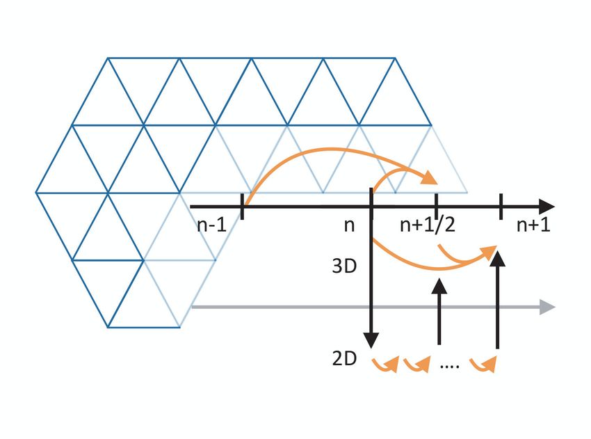
Zusammenfassung

Die Entwicklung und Implementierung von vorteilhaften Zeitschrittverfahren für
vorhandene Ozeanmodelle birgt das Potenzial, deren Ergebnis hinsichtlich höherer
numerischer Genauigkeit und geringerer numerischer Kosten bezogen auf erhöhte Sta-
bilität (größere mögliche Zeitschritte) zu verbessern. Stabilität und Genauigkeit von
Zeitschrittverfahren sollten im Kontext einer gekoppelten Raum-Zeit-Diskretisierung
betrachtet werden. Diesbezüglich ist die Herleitung und Analyse eines neuen
Zeitschrittverfahrens innerhalb der innovativen räumlichen Diskretisierung von
ICON-O (Ozeankomponente des Erdsystemmodells ICON) von bedeutendem In-
teresse.
In dieser Dissertation passen wir ein split-explizites Zeitschrittverfahren auf ICON-O
an und implementieren dieses. Damit gehen wir die beiden Punkte Genauigkeit und
Stabilität an: (a) Innerhalb überwiegend barotroper Experimente verringern wir den
Fehler, der durch die Ausbreitung eines barotropen Signals entsteht, um bis zu zwei
Größenordnungen. Zusätzlich wählen wir ein fortschrittliches Zeitschrittverfahren
für den baroklinen Zeitschritt und verbessern damit das barokline Signal für die für
uns relevanten, hohen Courant-Zahlen. (b) Die neue Raum-Zeit-Diskretisierung zeigt
eine 1.3-fach erhöhte numerische Stabilität für die ausgewerteten Experimente.
Zusätzlich zu dem neuem split-expliziten Zeitschrittverfahren, welches auf einem
Leap-Frog Adams-Moulthon-3 (LF-AM3) baroklinem Zeitschritt basiert, entwickeln
wir das split-explizite Zeitschrittverfahren für das in ICON-O ursprünglich mit einem
semi-impliziten Zeitschritt verwendete Adams-Bashfort-2 (AB2) Verfahren. Eine
der großen Leistungen dieser Arbeit war das Entwickeln dieser Zeitschrittverfahren
innerhalb der besonderen räumlichen Diskretisierung von ICON-O. Dieser folgend,
erhalten wir die Massen-Matrix, welche eine numerische Mode aufhebt, und erfüllen
diskrete Volumen- und Tracererhaltung.
In Experimenten mit ansteigender Komplexität vergleichen wir die zwei neuen split-
expliziten Raum-Zeit Diskretisierungen mit dem ursprünglichen semi-impliziten AB2
Verfahren. Wir zeigen die höhere Genauigkeit der barotropen Mode beider neuer
split-expliziten Verfahren anhand mehrerer Experimente von Schwerewellen. In einem
Lock-exchange Experiment zeigt sich, dass für kleine Courant-Zahlen beide split-
expliziten Verfahren aufgrund eines Kopplungsfehlers geringere Genauigkeit in der
Geschwindigkeit haben als das semi-implizite AB2 Verfahren. Dieser Kopplungsfehler
kann durch weiterführende Verbesserungen des split-expliziten Verfahrens vermieden
werden. Für die üblichen großen Courant-Zahlen ist die split-explizite LF-AM3
Raum-Zeit-Diskretisierung in der Geschwindigkeit genauer, sogar außerhalb des
Stabilitätslimits beider AB2 Verfahren. Zusätzlich ist LF-AM3 für Tracer, unabhängig

                                           iii
der Courant-Zahl, genauer. LF-AM3 zeigt ein etwas höheres numerisches Vermischen
von Tracern, auch beobachtbar bei der Verwendung kleinerer Zeitschritte in den
AB2 Verfahren. Wir begründen dies mit erhöhtem Rauschen in der Geschwindigkeit
auf Gitterskala, bedingt durch eine geringere numerische Geschwindigkeitsdiffusion.
Daraus ergibt sich für den Nutzer von ICON-O wiederum eine erhöhte Kontrolle über
die gesamte Diffusion der Geschwindigkeit. Innerhalb der Raum-Zeit-Diskretisierung
von ICON-O zeigt die neue split-explizite LF-AM3 Diskretisierung ein 1.3-fach höheres
Stabilitätslimit als das semi-implizite AB2 Verfahren und bis zu 1.5-fache erhöhte
Stabilität als die neue split-explizite AB2 Diskretisierung in den durchgeführten
Experimenten.

                                         iv
Contents

1 Introduction                                                                           1
   1.1   Ocean circulation modelling . . . . . . . . . . . . . . . . . . . . . . .       1
   1.2   Time discretization in ocean models . . . . . . . . . . . . . . . . . .         2
   1.3   Spatial discretization . . . . . . . . . . . . . . . . . . . . . . . . . . .    5
   1.4   Software development . . . . . . . . . . . . . . . . . . . . . . . . . .        5
   1.5   Thesis overview . . . . . . . . . . . . . . . . . . . . . . . . . . . . . .     5

2 Ocean model equations and spatial discretization                                      9
   2.1   Governing equations . . . . . . . . . . . . . . . . . . . . . . . . . . .       9
   2.2   Spatial framework of ICON-O . . . . . . . . . . . . . . . . . . . . . .        10
         2.2.1   Grid and variables . . . . . . . . . . . . . . . . . . . . . . . .     11
         2.2.2   Discrete reconstruction differential operators . . . . . . . . .       11
         2.2.3   Continuity equation . . . . . . . . . . . . . . . . . . . . . . .      13
         2.2.4   Tracer equation . . . . . . . . . . . . . . . . . . . . . . . . . .    14

3 Discrete split-explicit space-time discretization                                     15
   3.1   Barotropic-baroclinic mode splitting . . . . . . . . . . . . . . . . . .       15
   3.2   Time-stepping schemes . . . . . . . . . . . . . . . . . . . . . . . . . .      17
   3.3   Implications from continuity equation and tracer equation . . . . . .          19
   3.4   Volume and tracer conservation . . . . . . . . . . . . . . . . . . . . .       21
   3.5   Time stepping the barotropic system . . . . . . . . . . . . . . . . . .        21
   3.6   Averaging over the barotropic solution . . . . . . . . . . . . . . . . .       23
   3.7   Time stepping the baroclinic system . . . . . . . . . . . . . . . . . .        26
         3.7.1   LF-AM3 . . . . . . . . . . . . . . . . . . . . . . . . . . . . . .     26
         3.7.2   Adams-Bashfort-2 (AB2) . . . . . . . . . . . . . . . . . . . .         29
         3.7.3   Coupling error of the barotropic update . . . . . . . . . . . .        30

                                            v
4 Experiments and analysis                                                             33
  4.1   Diagnostics . . . . . . . . . . . . . . . . . . . . . . . . . . . . . . . .    34
        4.1.1   Error norms . . . . . . . . . . . . . . . . . . . . . . . . . . . .    34
        4.1.2   Reference potential energy (RPE) . . . . . . . . . . . . . . .         34
        4.1.3   Isolated terms . . . . . . . . . . . . . . . . . . . . . . . . . . .   35
  4.2   Gravity wave . . . . . . . . . . . . . . . . . . . . . . . . . . . . . . .     37
        4.2.1   Gravity wave in 1D . . . . . . . . . . . . . . . . . . . . . . . .     37
        4.2.2   Gravity wave on an aqua planet . . . . . . . . . . . . . . . .         40
        4.2.3   Gravity wave in 2D over an ocean mound . . . . . . . . . . .           41
  4.3   Lock-exchange . . . . . . . . . . . . . . . . . . . . . . . . . . . . . .      43
  4.4   Overflow . . . . . . . . . . . . . . . . . . . . . . . . . . . . . . . . . .   53
  4.5   Discussion . . . . . . . . . . . . . . . . . . . . . . . . . . . . . . . . .   53

5 Summary and outlook                                                                  57

References                                                                             61

                                           vi
Chapter 1
Introduction
1.1 Ocean circulation modelling
Ocean circulation models are of significant importance for oceanic and climate
research. They help us understanding processes like the energy transport within
the ocean or are needed for climate projection simulations (see e.g. Pörtner et al.
(2019)). In current research, ocean circulation models are well established, using a
large variety of numerical approaches. As such, there is ongoing research to improve
these models in many aspects, including for example the choice of a horizontal mesh
including grid staggering (Korn and Danilov, 2017), the advection scheme (Bernard
et al., 2006), the choice of the vertical coordinate (Chassignet et al., 2006; Adcroft
and Campin, 2004) and the parameterization of subgridscale processes (Griffies et al.,
2010a). In particular, accuracy of the model and numerical costs are two main
connected aspects in the development of the numerical schemes.
In ocean climate modelling mesocale eddies are of order 10km-100km and are often
not well resolved by the numerical grid. However, since they are the most energetic
eddies it is of particular interest to improve their representation in numerical models
(Griffies et al., 2010a). Higher accuracy can reduce the numerical diffusion and
therefore the damping of these mesoscale eddies. This higher accuracy can be
achieved for example by using a higher resolution of the ocean grid or using a
higher-order advection scheme. This however results generally in higher numerical
costs. These costs become even more crucial in simulations with high resolution like
mesoscale simulations which are performed on parallel high-performance computing
systems (Koldunov et al., 2019).
The ocean circulation model used in this study is ICON-Ocean (ICON-O) Korn
(2017), the ocean part of the new earth system model ICON-ESM (see e.g. Giorgetta
et al. (2018), Crueger et al. (2018)) of the Max Planck Institute for Meteorology.
There, the time-stepping is a semi-implicit Adams-Bashfort 2 (AB2) scheme. In
this thesis, we adapt the split-explicit time-stepping scheme from Shchepetkin and
McWilliams (2005) for the mathematical framework of ICON-O (Korn, 2017), which
is also applied to the ocean parameterizations in Korn (2018). Based on both the
time-stepping scheme from Shchepetkin and McWilliams (2005) and the spatial
discretization from (Korn, 2017), we develop a new space-time discretization with
the aim to increase desired larger numerical accuracy and higher stability.
11.2 Time discretization in ocean models
In general, time-dependent differential equations can be solved explicitly or implicitly
(Durran, 2013). To illustrate this difference, we consider the time derivative of an
arbitrary function ∂t f (t) = G(t) in simple discrete forms.
Explicit time-stepping For an explicit time-step, the right hand side G(t) of a
time-step tn is only dependent of the previous time-step tn−1 or older time-steps.
For such explicit time-step, the discrete time-derivative of a time-step size ∆t can be
written as
ft+∆t − ft
= G(f (t), f (t − ∆t), ..., t, t − ∆t, ...). (1.2.1)
∆t
The function at the new time step ft+∆t can be calculated as
ft+∆t = ft + ∆t G(f (t), f (t − ∆t), ..., t, t − ∆t, ...). (1.2.2)
The scheme in equation (1.2.2) describes the Euler scheme if the right hand side is
only dependent on the previous time step G = G(f (t), t).
For an explicit scheme, the Courant-Friedrichs-Lewy (CFL) stability criterion de-
scribes a stability limit αmax . The CFL criterion gives an upper time-step limit
∆tmax which the time-step ∆t may not exceed for a fixed grid space ∆x and a velocity
c. Hence in 1D, the CFL criterion can be written as
c∆t
≤ αmax . (1.2.3)
∆x
For a larger time step than ∆tmax , the model becomes unstable.
Implicit time-stepping In contrast to an explicit time-stepping scheme, for the
implicit time-stepping the right hand side is dependent on the new time step
ft+∆t − ft
= G(f (t + ∆t), t + ∆t). (1.2.4)
∆t
An implicit scheme is unconditionally stable, which means that it does not have
a stability limit like the CFL criterion. However, solving equation (1.2.4) is more
challenging and computationally more expensive than solving the explicit time-step
of equation (1.2.3) with the same time step size (Durran, 2013).
Time scales in the ocean Ocean dynamics are governed by modes on many
different time scales. The fastest acoustic modes are filtered out in hydrostatic
models such as considered for this thesis. One can broadly distinguish between
two main modes that remain in hydrostatic ocean models: On the one hand are
barotropic gravity waves (≈ 200 m/s). They are about two orders of magnitude
faster than, on the other hand, the fastest baroclinic modes, i.e. internal gravity
waves (≈ 1m/s) (Higdon and de Szoeke, 1997; Griffies et al., 2000).
21.2. TIME DISCRETIZATION IN OCEAN MODELS
In a flat-bottom ocean, a decomposition of the flow field into vertical eigenmodes,
including the barotropic mode as well as baroclinic modes, is straightforward (Gill,
1982). This decomposition is less trivial in a realistic ocean with full topography.
Nevertheless, also here, one can define the barotropic mode as the depth-averaged
flow and the baroclinic mode as the deviation hereof (Griffies et al., 2000).
One goal of time discretizations in global ocean models is to have an explicit time step
constrained by the baroclinic modes and not by the fast barotropic waves. Hence, the
baroclinic modes determine the maximum time step which we name in the following
baroclinic time step. Implicit time-stepping schemes are not used for the baroclinic
time-step due to high numerical costs. Constraining the time step to the barotropic
mode would lead to very small time steps and too high computational costs. The
depth-averaged barotropic flow is of lower dimension (2D) compared to the baroclinic
flow (3D) which can be exploited by solving the barotropic mode separately from
the baroclinic dynamics (Higdon and de Szoeke, 1997).
Early models used a rigid lid streamfunction method (Bryan, 1969), in which the
ocean surface is fixed and the barotropic dynamics are prevented. With further
development of ocean models, the free-surface is considered (see e.g. Maier-Reimer
et al. (1982)) and two different methods to primitive ocean equations have been
established (Griffies et al., 2000).
Semi-implicit time-stepping One way is to calculate the barotropic dynamics
implicitly while calculating the baroclinic dynamics explicitly. Such a semi-implicit
approach is used in ICON-O Korn (2017) or in Marshall et al. (1997). This approach
has several drawbacks, such as large numerical dissipation for the barotropic dynamics
due to the large implicit barotropic time step.
While the representation of barotropic dynamics for the general circulation (and
hence the large-scale climate) was considered not overly important for example by
McWilliams (1996), this view has changed nowadays. In particular, since we know
that mixing induced by barotropic tides is crucial for the global ocean circulation
(Wunsch and Ferrari, 2004) and that also the geographical distribution of this mixing
matters (e.g. Vic et al. (2018), MacKinnon et al. (2017)), an accurate representation
of the barotropic mode receives more and more attention.
Furthermore, such an semi-implicit approach requires a linear elliptic equation to
be solved which needs global communication for solving on multiple cores. This
differs from the explicit scheme, where only the information of the next neighbor is
needed. This global communication is supposed to be a bottleneck if simulations are
performed on large numbers of cores which are needed for high resolution simulations.
Split-explicit time-stepping A different approach is a split-explicit time-stepping
as in early work of Killworth et al. (1991), Bleck and Smith (1990) or Higdon and
de Szoeke (1997). There, the baroclinic dynamics are stepped forward with one large
baroclinic time-steps ∆t. The barotropic dynamics are also solved explicitly, but
with M small time-steps ∆t∗ = ∆t/M . The barotropic velocity is first obtained
by vertically averaging over the 3D momentum equation. Similarly, a barotropic-
baroclinic coupling terms is obtained by vertically averaging over the slow-changing
terms of the momentum equation. This term acts as a forcing term within barotropic
3dynamics. After the 2D subcycling of the barotropic dynamics, the barotropic
velocity is coupled back to the 3D velocity.
One advanced split-explicit time-stepping scheme has been developed for the Regional
Ocean Modeling System (ROMS) in a profound analysis of various time stepping
schemes with focus on accuracy and stability (Shchepetkin and McWilliams, 2005,
2009). This time-stepping scheme uses a Leap-Frog Adams-Moulthon-3 (LF-AM3)
scheme for the baroclinic step and the Adams-Bashfort-3 Adams-Moulthon-4 (AB3-
AM4) scheme for the barotropic system. Within ROMS, the LF-AM3 scheme is also
used with a non-hydrostatic version of ROMS (Kanarska et al., 2007). Lemarié (n.d.)
(note at CROCO website) gives a detailed description of the time-stepping algorithm
for CROCO, which is based on ROMS. The LF-AM3 scheme is nowadays also used
in NEMO Madec (2016) and for coastal flows in Kärnä Tuomas et al. (2013). Besides
Kärnä Tuomas et al. (2013), where discontinuous Galerkin finite elements are used
for an unstructured mesh, all previously mentioned models use structured grids.
Computational efficiency, stability and accuracy A larger possible Courant
number/time-step size usually decreases the computational costs since fewer time
steps have to be calculated for the same simulation time. The CFL criterion for
the explicit time-steps varies with the dynamics and depend on the space-time
discretization (Lemarié et al., 2015).
In Shchepetkin and McWilliams (2005) and Shchepetkin and McWilliams (2009),
where the time-stepping scheme for ROMS is developed, the stability and accuracy are
calculated based on a von Neumann linear stability analysis (Durran, 2013). While
LF-AM3 shows high stability, the AB2 scheme is asymptotically unstable. However,
only the time-discretization itself was analysed. An analysis of time-stepping schemes
which considers a coupled space-time discretization is given in Lemarié et al. (2015).
The analytical CFL number varies, depending on the advection scheme. For the
second-order centered advection scheme, the stability of the LF-AM3 scheme is
roughly 3 times larger than for the AB2 scheme. However, for a third-order upwind
scheme, the stability of LF-AM3 is only 1.5 times larger than for AB2.
Soufflet et al. (2016) compare ROMS with NEMO Madec (2016) in a suit of baroclinic
jet test cases. In this study, NEMO uses a Leapfrog temporal scheme with a modified
Robert-Asselin filter (Leclair and Madec, 2009). There, ROMS, using the split-
explicit time-stepping scheme as in Shchepetkin and McWilliams (2005), shows
higher computational efficiency, including larger stability. Furthermore, it shows
better results, presumably due to higher-order temporal and spatial discretization,
for the effective resolution which defines the range upon which numerical dissipation
becomes dominant.
For future high-resolution simulations which are run largely parallelized with thou-
sands of cores, computational efficiency becomes even more important than it is
today. This includes the scalability of the models as is investigated for example in
Koldunov et al. (2019) for FESOM2 (Danilov et al., 2017), or Ward and Zhang (2015)
for MOM from Spence et al. (2014). Solving the free-surface implicitly as done in
Korn (2017) with the GMRES solver causes global communication. The CG solver
shows increased scalability and is therefore more suitable Adamidis et al. (2011),
but still causes this global communication. This is a bottleneck of the numerical
41.3. SPATIAL DISCRETIZATION
efficiency of high-resolutions simulations where many cores are used. Split-explicit
schemes do not have global communication which is one reason why they are widely
used.
1.3 Spatial discretization
Lemarié et al. (2015) perform a space-time stability analysis of the LF-AM3 and
AB2 schemes within ROMS, which uses a structured grid. Instead, ICON-O uses
an unstructured icosahedral grid with C-type staggering for the variables, where
scalars are defined on cells centers and velocities are defined on edge midpoints.
ICON-O uses a unique mathematical framework described in Korn (2017) which is
also used for a shallow-water model in Korn and Linardakis (2018). In ICON-O,
discrete methods from Finite Elements, Finite Volume and Mimetic Finite Differences
are used. However, using C-type staggering on an unstructured grid leads to an
undesired computational grid mode (Danilov, 2010; Gassmann, 2011). This grid
mode appears since the degrees of freedom of scalar variables on cells is different
from vector variables such as velocities which are defined on edges Danilov (2013).
The grid mode has to be treated globally for an ocean model. For the icosahedral
grid with C-type staggering, possibilities to control the grid mode are damping (Wan
et al., 2013; Zängl et al., 2015), or filtering, (Wolfram and Fringer, 2013). However,
these approaches result in an inconsistent continuity formulation. Instead ICON-O
uses a mass-matrix which especially appears in the continuity equation where the
grid mode is filtered out (Korn, 2017).
1.4 Software development
The development of the split-explicit time-stepping schemes within ICON-O required
changes of the code throughout the dynamical core. The barotropic subcycling as
well as the 2-step LF-AM3 scheme required many new routines, operators and overall
changes. Even more, in ICON-O, the time-stepping scheme is embedded deeply
within the code and spread over many routines. Therefore, a proper implementation
within the code was one major effort of the development of the new split-explicit
time-stepping schemes which included changes in the order of 10000 codes lines.
Due to the depth of code changes within ICON-O, we have not fully parallelized the
new split-explicit time-stepping schemes. Therefore, we did not simulate numerically
expensive experiments such as eddy resolving experiments as shown in for example
Soufflet et al. (2016) and Petersen et al. (2015). Instead, we focus mainly on idealized
2D experiments in chapter 4, which are numerically less expensive.
1.5 Thesis overview
The new time-stepping scheme that we develop in this thesis is consistent within the
novel space discretization of the C-type staggered icosahedral grid of ICON-O Korn
(2017). The split-explicit time-stepping scheme of Shchepetkin and McWilliams (2005)
is the main time-stepping scheme of our choice since it has superior stability and
5accuracy towards other schemes (Lemarié et al., 2015; Soufflet et al., 2016). Therefore,
we use LF-AM3 for the baroclinic step and AB3-AM4 for the barotropic step similar
to Shchepetkin and McWilliams (2005). Formulating this time-stepping scheme
within the spatial framework of ICON-O, we derive a new space-time discretization
which is the first split-explicit scheme of a C-type staggered icosahedral grid. We
ensure conservation properties while retaining the mass-matrix which filters out the
grid-mode as motivated in the previous section 1.3.
Additionally to using the LF-AM3 predictor-corrector scheme for the baroclinic
step, we adapt the original AB2 scheme of Korn (2017) to be used together with
the AB3-AM4 barotropic subcycling. This gives us the opportunity to compare a
split-explicit and semi-implicit scheme with the same AB2 baroclinic step as well as
different split-explicit schemes of the baroclinic step with the same subcycling.
The baroclinic solution is updated with a fast-time averaged barotropic solution
to avoid aliasing, to achieve second-order accuracy and for consistency within the
discrete framework (Shchepetkin and McWilliams, 2005). We show that the solution
of the fast-time averaging which is used to update intermediate velocity values
introduces a coupling error that can be avoided, if the centroid of this averaging is
equal to the predicted (LF-AM3) or weighted (AB2) velocity.
After diagnostic tests, we analyse accuracy and stability in idealized tests with
increasing complexity. We show higher accuracy of the split-explicit schemes for
various gravity wave tests. While the lock-exchange test and the overflow test are
used to compare mixing between different models in Ilicak et al. (2012) and Petersen
et al. (2015), we use these tests to compare different space-time discretizations of the
same model. We use the lock-exchange test to analyse mixing and accuracy of the
different time-stepping schemes. Further, we introduce a reduced vertical resolution
which we use to analyse the stability. Lastly, we compare the results that we get to
other space-time discretizations which are discussed in Lemarié et al. (2015).
This thesis is structured as follows. First, we give an overview of the ocean model
equations and the spatial framework as introduced by Korn (2017), which is the
basis of our new space-time discretization (chapter 2). There, we also give the
discrete continuity equation of Korn (2017), which is kept for the new split-explicit
time-stepping scheme.
We derive the new split-explicit space-time discretization in chapter 3. We show the
continuous split-explicit form of the momentum equation and discuss the main parts
of the time-stepping algorithm. We summarize all time-stepping schemes that we
use.
We retain the original continuity equation and tracer equation consistently within
our framework and we therefore guarantee volume and tracer conservation. Based
on implications of the discrete continuity equation, we derive the new space-time
discretization of the barotropic system and show a temporal averaging over the
barotropic solution consistent within our spatial framework. We finalize the new
space-time discretization of the discrete baroclinic step based on the LF-AM3 scheme
and the discrete baroclinic step based on the AB2 scheme including a discussion of a
coupling error.
In chapter 4, we analyse and discuss the new LF-AM3 and AB2 split-explicit time-
stepping schemes and compare them to the old-time-stepping scheme qualitatively
61.5. THESIS OVERVIEW
and quantitatively with experiments of increasing complexity. For the analysis, we use
error norms and the reference potential energy (RPE) as diagnostic tools. Simulations
where we isolate the terms of the right-hand side of the momentum equation give us
confidence in the new split-explicit algorithms which includes mode-splitting and the
update of the baroclinic step.
We analyse the improvements of the split-explicit schemes compared to the semi-
implicit scheme for highly barotropic dynamics for different gravity wave experiments.
As expected, the split-explicit time-stepping schemes are more accurate since the
barotropic dynamics are well resolved compared to the AB2 semi-implicit scheme.
We analyse diapycncal tracer diffusion, accuracy and stability in the lock-exchange
experiment in which baroclinic dynamics are dominant compared to the barotropic
dynamics. For low Courant numbers (small time step sizes), a mode-splitting
error causes a decrease in accuracy for the split-explicit schemes. We introduce a
configuration of the lock-exchange experiment with reduced vertical resolution so
that we can analyse the stability and accuracy for relevant large Courant numbers
near the stability limit. There, the LF-AM3 scheme is more accurate and shows
larger stability than both AB2 schemes. Also, we see a slight increase of diapycnal
diffusion for the LF-AM3 scheme. We relate this to higher accuracy and therefore a
decrease of total diffusion which otherwise damps small scale noise which causes the
diapycnal diffusion (Ilicak et al., 2012).
We discuss implications of the coupling error and relate the gain of stability of the
LF-AM3 scheme to other space-time discretizations in Lemarié et al. (2015). We
argue that due to the unstructured icosahedral grid, the gain of stability of the
LF-AM3 scheme compared to the AB2 schemes differs from the gain achieved in
other space-time discretizations shown in Lemarié et al. (2015).
Finally in chapter 5 we summarize the results and give a potential outlook of the split-
explicit time-stepping included in ICON-O as well as potential future experiments to
compare the different schemes.
78
Chapter 2

Ocean model equations and
spatial discretization

The governing primitive ocean equations that we summarize in section 2.1 are the
underlying equations that we solve. As motivated in section 1.3, a novel spatial
discretization of the primitive ocean equations on a C-type staggered icosahedral
grid is derived in Korn (2017). We will formulate the split-explicit time-stepping
schemes based on this spatial discretization. We summarize the discrete spatial
framework of ICON-O (Korn, 2017) in section 2.2. We discuss all variables and
operators that we need for the discrete split-explicit discretization. Furthermore, we
show the discrete continuity equation and the discrete tracer equation of ICON-O
which we keep unchanged for the new split-explicit time-stepping scheme.

2.1     Governing equations

Independent of the new time-stepping scheme, we solve the primitive ocean equations
in the same vector invariant form as in ICON-O (Korn, 2017) which are given in e.g.
Müller (2006)

      ∂v                    ∇h |v|2    ∂v   1              ∂ v ∂
         + (f + ω)z × v +           +w    + ∇h p − D h v −    A    v = 0,
      ∂t                        2      ∂z ρ0               ∂z   ∂z
                                                                         (2.1.1a)
      ∂p
          = −ρg,                                                         (2.1.1b)
      ∂z         Z η
      ∂η
         + divh        vdz = 0,                                           (2.1.1c)
      ∂t           −H
               ∂w
      divh v +      = 0,                                                 (2.1.1d)
               ∂z
      ∂c                                ∂ C ∂
         + div(Cv) − divh (KC ∇h C) −     A    C = 0,                     (2.1.1e)
      ∂t                               ∂z   ∂z
      ρ = Feos (p, T, S).                                                 (2.1.1f)

                                          9
Here, v is the horizontal velocity, w the vertical velocity, η the free surface height,
ω the vorticity, f the Coriolis parameter, C are the tracer quantities temperature
T and salinity S, ρ is the water density, ρ0 the reference density, p the hydrostatic
pressure and g the gravitational constant. Dh is the horizontal velocity diffusion,
Av the vertical velocity diffusion coefficient, KC the horizontal and AC the vertical
diffusion for a tracer C. Feos is the equation of state. ~z is the vertical direction
vector, ∇h the horizontal differential operator and divh the horizontal divergence.
With the decomposition of the pressure p = phyd + ps into the sum of the internal
hydrostatic pressure phyd and the surface pressure ps = gρ0 η(x, y, t), equation (2.1.1a)
becomes
∂v ∇h |v|2 ∂v 1
+ (f + ω)z × v + +w + ∇h phyd + g∇h η(x, y, t)
∂t 2 ∂z ρ0 (2.1.2)
∂ v ∂
− Dh v − A v = 0.
∂z ∂z
The boundary of the ocean ∂Ω can be divided into the boundary at the surface ∂ω s ,
at the bottom ∂ω b and at the lateral boundaries ∂ω l . The boundary conditions for
the velocity are
∂v ∂v
Av = τ at ∂Ωs , Av = Cb |v|v at ∂Ωb ,
∂z ∂z (2.1.3)
t ∂η
v = 0 at ∂Ω , w = 0 at ∂Ωb , w = at Ωs .
∂t
Here, τ is the wind stress, tangential to the ocean. Cb is the bottom drag coefficients.
The boundary conditions for the tracers are
∂C ∂C
KC = −QC at∂Ωs , = 0 at∂Ωb , ∇h C = 0, at∂Ωt . (2.1.4)
∂z ∂z
Here, QC is the surface flux for each individual tracer C. In the idealized experiments
in chapter 4 no bottom friction and surface forcing are used for the velocity and
tracers. Hence, the only boundary condition that is used in the experiments is
the lateral boundary condition of the velocity and tracers for the gravity wave test
over an ocean mound in section 4.2.3, the lock-exchange test in section 4.3 and the
overflow test in section 4.4.
2.2 Spatial framework of ICON-O
In this section, we summarize necessary parts of the discrete spatial framework of
ICON-O that we use for the new discretization in chapter 3. More comprehensive
details, especially regarding the mathematical framework, can be found in Korn
(2017). We define all variables in section 2.2.1 and all operators in section 2.2.2 that
we need for the new split-explicit time-discretization. Besides the needed operators
given in Korn (2017), we define one new reconstruction operator that is needed
during the barotropic subcycling.
102.2. SPATIAL FRAMEWORK OF ICON-O
Furthermore, we show the same discrete continuity equation in section 2.2.3 and the
discrete tracer equation in section 2.2.4 as given in Korn (2017). Later, in section
3.3, we derive the new split-explicit time-stepping scheme consistent to this discrete
continuity equation. Then, by keeping the discrete continuity equation and the
discrete tracer equation in the same form as given in Korn (2017), we immediately
guarantee volume and tracer conservation as well as constancy preservation as we
discuss in sections 3.3 and 3.4.
2.2.1 Grid and variables
In ICON-O, an icosahedral grid is used with a C-type staggering of the variables.
Different vertical levels are denoted with, k ∈ {1, 2, ..., kbot }, whereas k = 1 denotes
the surface layer and k = kbot the layer at the bottom of the ocean.
Each edge e of the triangle has a normal vector ~ne,k and a tangential vector ~te,k .
For an edge between two neighbouring cells Kk and Lk , the edge midpoint is at
~xek = ~xK|L,k with cell midpoints ~xK,k and ~xL,k . The cell volume of a cell K is
denoted as |K|. The length of an edge e between two cell midpoints K and L is
|e| = |K|L| and the length between the cell midpoints is |e⊥ | = |K|L⊥ |.
For the vertical grid, a z-level coordinate system is used. As such, apart from the
surface layer which changes with the free-surface, all cells K at layer k have a constant
thickness of ∆zK,k . The same holds for the thickness ∆ze.k at edge e.
With the C-type staggering, the velocities are defined as their normal component
on a cell edge ve,k = ~ve,k · ~ne,k . Scalars such as tracer values are defined on cell
midpoints.
The cells and edges of the icosahedral grid define a so-called primal grid. Connecting
the cell midpoints of the icosahedral grid results in a dual grid consisting of hexagons
and pentagons (which only appear in a spherical grid and not in a regular grid such
as a channel). The edges of the dual grid are called dual edges and cell centers of the
dual grid are defined on the vertices of the icosahedral grid. The primal grid and the
dual grid become relevant in the description of the spatial operators in the following
section 2.2.2.
2.2.2 Discrete reconstruction differential operators
The discrete framework of ICON-O is based on a discrete space for normal velocities
on edges and scalars on cells on the primal grid and a discrete space for scalars on
cells on the dual grid. These spaces are endowed by volume weighted scalar products
for scalar and vector quantities. Reconstruction operators as well as differential
operators map quantities from one space to the other. For example, the result of the
discrete divergence of the velocities is defined on cell centers whereas the velocities
are defined on edges. Hence, the divergence maps vectors, defined at edges, to cell
centers. Additionally, the discrete scalar products are used to derive transposed
operators as for example the discrete gradient which is derived from the discrete
divergence.
We want to emphasise, that this framework is defined in Korn (2017), where more
mathematical details and explanation of this mathematical framework can be found.
11In the following, we only show the operators which are used in this thesis and omit
details such as the notation of the scalar product.
Discrete reconstruction operators A reconstruction operator P maps normal
velocities on edges to velocity vectors on cells
1 X
v → P vK,k := ve,k |e|(~xe − ~xK )∆ze,k , (2.2.1)
|K|∂zK,k
e∈∆K
while a transposed reconstruction operator maps cell velocities to edges
1
~vK,k · (~xK|L,k − ~xK ) − ~vL,k · (~xK|L,k − ~xL ) , if K|L ∈
/ ∂Gk .
:= |K|L |
T ⊥
~v → P ~vK|L,k
0 else
(2.2.2)
Here, ∂Gk describes the discrete lateral boundary of the domain Ω and describes a
partial set of all edges E which belong to water cells
∂G := {ek = Kk |Lk ∈ E : exactly one of the cells Kk or Lk
which is adjacent to the edge ek
is a land cell and the other one is a water cell}.
In addition to Korn (2017), we define a new reconstruction operator P ∗ which is
similar to the reconstruction operator P , but independent of the thickness on cells
and edges
1 X
v → P ∗ vK := ve |e|(~xe − ~xK ). (2.2.3)
|K|
e∈∂K
We use this new operator for a re-formulation of the discrete continuity equation and
within the discrete barotropic momentum equation.
The reconstruction operator P reconstructs a vector in a cell center out of vectors
defined on the icosahedral grid. By contrast, a dual reconstruction operators P̂
reconstructs a vector at the cell center of the dual grid K̂, at ~xK̂
1 X
v → P̂ vK̂,k := ve,k |e⊥ |∆ze,k ~ze,k × (~x∗e,k − ~xK̂,k ). (2.2.4)
|K̂|∆zK̂,k
e∂ K̂k
Here, ~x∗e,k is the midpoint of the dual edge.
The transposed operator of the dual reconstruction operator reconstructs vectors at
vertices to edge values
h i
1
~vK̂,k · (~x∗K̂ − ~xK̂k ) − ~vL̂k · (~x∗K̂ − ~xL̂k ) , if K̂|L̂ ∈
/ ∂Gk
v → P̂ † vK̂k |L̂k := |K̂k |L̂⊥
k| k |L̂k k |L̂k
0 else.
(2.2.5)
122.2. SPATIAL FRAMEWORK OF ICON-O
By applying the transposed reconstruction operator P T of equation (2.2.2) after the
reconstruction operator of P of equation (2.2.1), the mass matrix, a positive definite
operator MG ve,k := P T P ve,k is defined. MG maps edge quantities to the cells and
back to the edges e. We also define the operators MG [f, v]e,k := P t (f P v)e,k as a
product of a scalar quantity f at cell centers with normal velocities at the edges.
Similarily, we define M̂G [fˆ, v]e,k := P̂ † (fˆP̂ v)e,k where fˆ is a scalar quantity on the
dual grid.
Additionally, we define the layer-thickness-independent mass matrix M∗G := P T P ∗ .
M ∗ is new compared to the original framework and needed for the vertically integrated
flux and during the barotropic subcycling. Note, that by using P ∗ for this mass
matrix, M∗G is similar to the discrete formulation of Korn and Linardakis (2018),
where the shallow-water equations are solved with the same discrete approach as in
Korn (2017).
Discrete differential operators The discrete divergence of the velocity divvK,k
in a cell K of the vertical level k uses edge velocities ve,k and is a mapping from
edges to cells
1 X
div vK,k := ve,k |e|ne,K ∆ze,k . (2.2.6)
|K|∆zK,k
e∈∂K
Similar to the transposed reconstruction operators, the discrete gradient grad of
a scalar quantity fK|L,k between the cells K and L at the vertical level k can be
derived from the divergence and is a mapping from cells to edges
fK,k − fL,k
gradfK|L,k := . (2.2.7)
|K|L⊥ |
The curl is a mapping from the primal grid to the dual grid
1 X
curl vK̂,k := ve,k |ê|te,k ∆ze,k . (2.2.8)
|K̂|∆zK̂,k
e∈∂ K̂
The vertical differential operator between two vertical levels k and k + 1 to a half-level
k + 1/2 is
fK,k − fK,k+1
Dz fK,k+1/2 := . (2.2.9)
∆zk
2.2.3 Continuity equation
With the discrete differential operators from the previous section 2.2.2, the divergence
free continuity equation from equation (2.1.1d) is discretized to
wK,k − wK,k+1
Dz wK,k = = −div (MG v)K,k . (2.2.10)
∆zK,k
Reformulating (2.2.10) and using the bottom boundary condition wkbot = 0, the
vertical velocity can be obtained
wK,k = wK,k+1 − div (MG [∆z, v])K,k , for k = kbot − 1, ..., 1. (2.2.11)
13By applying a vertical integral from the bottom layer kbot to layer k we can calculate
the vertical velocity as an integral over the horizontal mass fluxes
k−1
X
wK,k = − div (MG [∆z, v])K,k . (2.2.12)
k=kbot
This discretization that includes the mapping of the mass matrix MG filters out
the grid mode which results from the C-type staggering on the triangular grid
Korn (2017). This is a key feature which we have to consider for the split-explicit
time-stepping.
2.2.4 Tracer equation
Similar to the discrete continuity equation, we use the same discrete tracer equation
as derived in Korn (2017). The result of the discrete tracer equation is on cells. For
the ease of better readability, we omit the spatial indices in the following equation:
∂ (∆zC) h i
+divF(MG [∆zC, v])+Dz F ∆z C̃w +divKC gradC+DZ AC DZ C = FC .
∂t
(2.2.13)
Here, F is the Zalesak limiter, a horizontal flux limiter (Zalesak, 1979) used for
flux-corrected transport to achieve high accuracy, but to avoid over and undershoots
from the tracer flux.
This discrete tracer equation is a 1-step tracer scheme. In Shchepetkin and McWilliams
(2005), which our split-explicit time-stepping scheme is based on, a 2-step tracer
scheme is presented. There, Shchepetkin and McWilliams (2005) calculate intermedi-
ate tracer values at time step n + 1/2 with a focus on constancy preservation with the
loss of the conservation property. Still, their tracer corrector step is both constancy
preserving and conservative. Using a 2-step tracer scheme has the advantage, that
the corrector step not only uses predicted velocities at n + 1/2, but also intermediate
tracer values.
For simplicity and to be able to separately analyse changes in accuracy and stability
which result from a change of the momentum equation alone, we use the same discrete
tracer equation as derived for ICON-O (Korn, 2017). Therefore, we keep the tracer
values constant after the baroclinic LF-AM3 predictor step. Thus, we will use the
tracer values of n at n + 1/2 for the corrector step. Following Shchepetkin and
McWilliams (2005), a 2-step tracer scheme is a potential future option for the new
split-explicit time-stepping schemes. Then, a predictor step not only has to be added
within the calculation of the tracer values, but also within the routines of the Zalesak
limiter.
14Chapter 3
Discrete split-explicit
space-time discretization
Based on the discrete spatial framework, we derive a new discrete split-explicit
space-time discretization for the primitive ocean equations in this chapter. First,
we show the barotropic-baroclinic mode splitting in section 3.1, which is similarly
used for all split-explicit time-stepping schemes (see e.g. Killworth et al. (1991),
Bleck and Smith (1990) or Higdon and de Szoeke (1997)). Then, in section 3.2, we
describe all time-stepping schemes in generalized formulations, which we will use for
the baroclinic step and for the barotropic step of our new split-explicit space-time
discretization.
From section 3.3 on, we develop the new space-time discretization. We discuss in
section 3.3 that the continuity equation, which we keep from Korn (2017) (see section
2.2.3), defines the integrated velocity. Furthermore, we obtain a condition for a
slow-changing free-surface equation. Fulfilling this condition, we argue in section 3.4
that we fulfill volume and tracer conservation. We derive the new discrete space-time
discretization of the barotropic subsystem in section 3.5. We describe the fast-time
averaging over the barotropic solution from Shchepetkin and McWilliams (2005)
within our discretization in section 3.6. We show that we can fulfill the condition
from the continuity equation for the slow-changing free-surface with this fast-time
averaging within our new discretization. We finalize the new space-time discretization
with the discrete baroclinic step. We derive the new discrete LF-AM3 predictor-
corrector scheme (Shchepetkin and McWilliams, 2005) in section 3.7.1 and we briefly
describe in section 3.7.2 the discrete baroclinic step based on the AB2 step which is
used for the semi-implicit time-stepping scheme originally in ICON-O (Korn, 2017).
3.1 Barotropic-baroclinic mode splitting
As described in section 1.2, the differences in the time scales of the barotropic and
the baroclinic modes can be exploited by splitting the momentum equation into a
slow changing 3D baroclinic part and a fast changing 2D barotropic part as derived
in previous work e.g. (Killworth et al., 1991), Bleck and Smith (1990) or Higdon and
de Szoeke (1997). This mode-splitting is the basis for split-explicit time-stepping
15schemes. In this section, we show the barotropic-baroclinic splitting for a vertical
grid with z-coordinates. Vertical z-coordinates are used in ICON-O, where except
for the top layer with changing free-surface height, all cells of a layer have constant
thickness (Korn, 2017).
The total velocity v is separated into a baroclinic v 0 and a barotropic part v̄
v = v 0 + v̄. (3.1.1)
The barotropic velocity is obtained
R η by vertical integration over the velocity and
division over the total depth D = −H dz
1 η
Z
1
v0 = vdz = V̄ . (3.1.2)
D −H D
Here, −H denotes the depth of the ocean and V̄ the vertically integrated/barotropic
flux.
As such, the baroclinic velocity v 0 possesses no depth average
Z η
v 0 dz = 0. (3.1.3)
−H
Applying the vertical integral on the momentum equation (2.1.1a) results in the
equation of the barotropic flux
∂t V̄ + f z × V̄ = −gD∇h η + R, (3.1.4)
with
Z η
1 ∂v ∂ ∂
R= dz(− ∇h phyd − v · ∇h v − ωz × v − w + Dh v + Av v). (3.1.5)
−H ρ0 ∂z ∂z ∂z
Here, R is called the barotropic-baroclinic coupling term. It includes all nonlinear
terms and all terms which are slowly changing compared to the barotropic dynamics.
During the barotropic stepping, the barotropic-baroclinic coupling term R is kept
constant. The pressure-gradient term and the Coriolis term are the fast changing
terms and are used to calculate the barotropic dynamics besides the barotropic-
baroclinic coupling term. In newer models such as e.g. described in Ringler et al.
(2013), the Coriolis term is included for the barotropic system whereas only the
pressure gradient term is changed over the subcycling in e.g. Higdon and de Szoeke
(1997).
The equation for the barotropic velocity v̄ can be obtained by dividing the equation
for the barotropic flux (3.1.4) over the total depth
1
∂t v̄ + f z × v̄ = −g∇h η + R. (3.1.6)
D
Substituting the barotropic mass flux V̄ into the free surface equation (2.1.1c) gives
∂η
+ divh V̄ = 0. (3.1.7)
∂t
163.2. TIME-STEPPING SCHEMES
Combined, the equation for the barotropic flux (3.1.4) and the free-surface equation
(3.1.7) result in the fast 2D barotropic system.
Subtracting the barotropic momentum equation (3.1.6) from the momentum equation
(2.1.1a) gives the momentum equation for the baroclinic velocity
∂v 0 ∂v ∂v̄
= −
∂t ∂t ∂t
∇h |v|2 ∂v 1
= − ωz × v − f z × v 0 − −w − ∇h phyd
2 ∂z ρ0
∂ v ∂ 1
− g∇h η(x, y, t) + Dh v + A v+ R (3.1.8)
∂z ∂z D
1
= T − f z × v̄ + R (3.1.9)
D
Here, T is the complete right-hand side of the momentum equation (2.1.1a).
The vertical z-coordinate system allows us to split the pressure gradient term between
the internal dynamics and the external gravity wave highly accurately (Higdon and
de Szoeke, 1997). This allows us to easily differentiate between the fast changing
gradient of the free-surface and the slow changing hydrostatic pressure gradient. In
models with isopycnal or terrain-following coordinates this splitting has to be treated
carefully as to not lead to a large error which is called mode-splitting error (see e.g.
Shchepetkin and McWilliams (2005) or Higdon and de Szoeke (1997)).
3.2 Time-stepping schemes
In this work, we will use three different time-stepping schemes. For the baro-
clinic time step we compare the Adams-Bashfort-2 (AB2) scheme to the Leap-Frog
Adams-Moulthon-3 (LF-AM3) scheme. For the barotropic stepping we will use
the Adams-Bashfort-3 Adams-Moulthon-4 (AB3-AM4) scheme. We will use these
schemes similarly for the velocity and the free-surface height for the new space-time
discretization of the barotropic system later in section 3.5 and for the discretization
of the baroclinic momentum equation in section 3.7. Therefore, we denote the time
dependent functions which can be solved by the generalized formulations of the
time-stepping schemes with v and η.
Adams-Bashfort-2 The AB2 scheme which is originally used for the semi-implicit
time-stepping in Korn (2017) is based on Marshall et al. (1997). AB2 is an example
for a multistep method where the right-hand-side at time-step n is dependent on the
older time-step (here, time step n − 1). Similar to section 1.2, we consider the time
derivative of function ∂v(t)
∂t = G(v, t). The AB2 step is
n+1 n 3 n 1 n−1
v = v + ∆t + G − + G . (3.2.1)
2 2
The right hand side is extrapolated in between time step n and time step n + 1,
where a nonzero leads to an offset away from the midpoint n + 1/2. In ICON-O
(Korn, 2017), as well as in this thesis we choose = 0.1, since AB2 becomes unstable
for = 0 under inviscid conditions (Marshall et al., 1997).
17Leap-Frog Adams-Moulthon-3 (LF-AM3) Shchepetkin and McWilliams (2005)
investigate a variety of time-stepping schemes regarding accuracy and stability for a
linear hyperbolic system
∂v ∂η
= G(v, η, t), = F(v, η, t) (3.2.2)
∂t ∂t
∂η ∂v
where G = −c ∂x , F = −c ∂x and c is the phase speed. This system can be considered
as a simplified form of the coupled system of the momentum equation and the
free-surface equation of the primitive ocean equations which are shown in section 2.1.
For this system, Shchepetkin and McWilliams (2005) derive a generalized predictor-
corrector time-stepping scheme which can be simplified to a Leap-Frog Adams-
Moulthon-3 (LF-AM3) scheme. LF-AM3 originally has a Leap-Frog predictor step
and an Adams-Moulthon-3 corrector step. LF-AM3 can be reformulated (Shchepetkin
and McWilliams, 2005) to the predictor step
n+ 21 1 n−1 1
η = − 2γ η + + 2γ η n + ∆t (1 − 2γ) F n , (3.2.3)
2 2
1 1 1
v n+ 2 = − 2γ v n−1 + + 2γ v n + ∆t (1 − 2γ) G n , (3.2.4)
2 2
followed by the corrector step
1
η n+1 = η n + ∆t F n+ 2 , (3.2.5)
n+1 n n+ 21
v = u + ∆t G . (3.2.6)
Choosing γ = 1/12 results in third order accuracy and a large stability limit (c.f.
section 1.2) of αmax = 1.587 (Shchepetkin and McWilliams, 2005) and is also used in
e.g. Kärnä Tuomas et al. (2013). As a comparison, the AB2 scheme is asymptotically
unstable if it is analysed by following the linear stability analysis of Shchepetkin
and McWilliams (2005) similar to the analysis of LF-AM3. However, this analysis
does not consider the coupled space-time discretization where AB2 shows also finite
stability (Lemarié et al., 2015). This is expected since the AB2 scheme is successfully
used in ocean circulation models (Korn and Danilov, 2017; Marshall et al., 1997).
Still, also in the coupled space-time discretization, LF-AM3 shows larger stability
compared to AB2 (Lemarié et al., 2015).
Due to high stability and accuracy of the LF-AM3 scheme in Soufflet et al. (2016)
and Lemarié et al. (2015), we choose the LF-AM3 as the new alternative to the AB2
scheme for the baroclinic step by following the algorithmic approach of Shchepetkin
and McWilliams (2005).
We note that in this formulation the Leap-Frog step as well as the Adams-Moulthon-3
step are mixed together. The symmetry of the predictor step in equation (3.2.3)
and the corrector step in equation (3.2.5) of the LF-AM3 scheme is due to the
reformulation of the original LF-AM3 scheme. With this reformulation, especially
intermediate velocity values at time step n + 1/2 are obtained and are used for the
discrete LF-AM3 step later in section 3.7.1.
183.3. IMPLICATIONS FROM CONTINUITY EQUATION AND TRACER
EQUATION
Adams-Bashfort-3 Adams-Moulthon-4 (AB3-AM4) Similar to the gener-
alized predictor-corrector step which can be simplified to the LF-AM3 scheme,
Shchepetkin and McWilliams (2005) develop a generalized forward-backward scheme
with an Adams-Bashfort-3 like forward step and an Adams-Moulthon-4 like backwards
step. This AB3-AM4 scheme can be reformulated to (Shchepetkin and McWilliams,
2009)
n+1 n 3 n 1 n−1 n−2
η = η + ∆t +β F − + 2β F + βF , (3.2.7)
2 2
1 1
un+1 n
= u − ∆t + γ + 2 G n+1
+ n
− 2γ − 3 G + γG n−1
+ G n−2
.
2 2
(3.2.8)
Choosing the parameters β = 0.281105, γ = 0.088, = 0.013 is a compromise choice
within the linear stability analysis of Shchepetkin and McWilliams (2009) between
large stability and second-order accuracy. The stability limit is αmax = 1.7802
(Shchepetkin and McWilliams, 2009). AB3-AM4 is a suitable choice to solve the
barotropic system. Besides the stability and the second-order accuracy, it has large
dissipation for high velocities which filters out fast barotropic dynamics within the
nonlinear system that might lead to instabilities (Shchepetkin and McWilliams, 2009).
Additionally, compared to for example the LF-AM3 predictor-corrector scheme, AB3-
AM4 uses only one calculation step of the right-hand side which reduces numerical
costs.
3.3 Implications from continuity equation and tracer
equation
From this section on, we derive the new split-explicit space-time discretization. For
this new discretization, we have to ensure that the tracer fluxes are consistent with
the continuity equation which connects volume fluxes and tracer fluxes. This means
that using a uniform tracer field in the tracer transport equation (3.3.1) results in
the discrete continuity equation (2.2.10) (Korn, 2017). To show this consistency, we
closely follow the argumentation of Korn (2017). There, in the last step, the discrete
free-surface equation, which is solved by the implicit solver, ensures this consistency.
Similarly, for this split-explicit discretization, we derive a slow-changing free-surface
equation. However, we do not solve this equation since we solve the free-surface
during the barotropic subcycling. Instead, this slow-changing free-surface equations
gives us a constraint that the result of the barotropic subcycling has to fulfill to
ensure the consistency between the continuity equation and the tracer equation.
Additionally, this slow-changing free-surface equation defines the vertical integral
that we use to calculate the barotropic flux.
For the ease of better readability, we omit some indices of the right-hand side of
the following equations. Following Korn (2017), we consider a uniform tracer field
Ckn = C at time step n for all cells K. With this, the discrete tracer equation (2.2.13)
19Sie können auch lesen